---

一、实验概览

对于这次lab，实现的主要是基于 cost-based optimizer（基于成本的优化器）。在此之前笔者先补充一些概念。
拿Mysql来说，一条sql的执行步骤主要为以下的图：

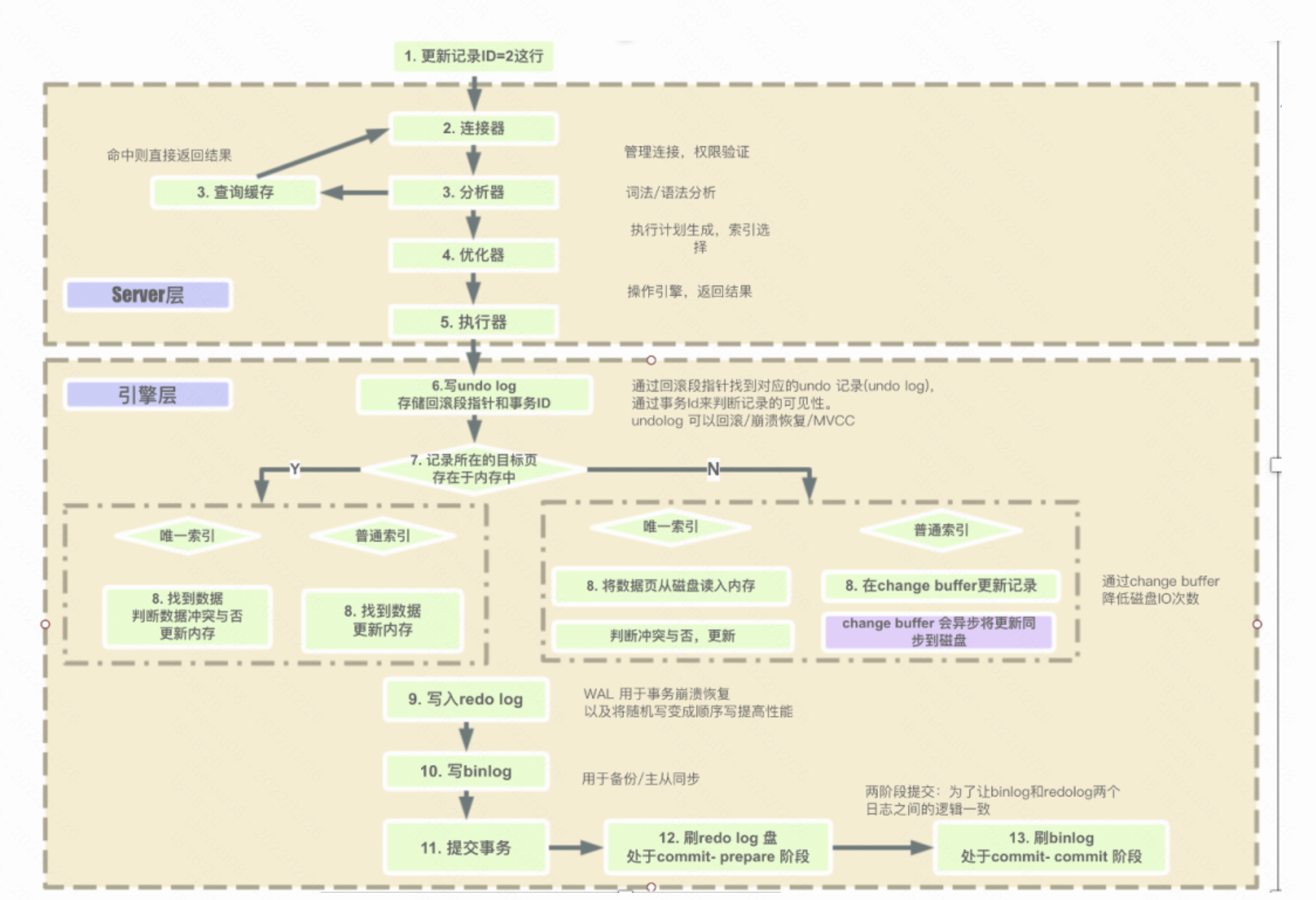
而本次lab要实现的也就是优化器这一步。

• 此阶段主要是进行SQL语句的优化，会根据执行计划进行最优的选择，匹配合适的索引，选择最佳的执行方案。

比如一个典型的例子是这样的：

• 表T，对A、B、C列建立联合索引，在进行查询的时候，当SQL查询到的结果是：select xx where B=x and A=x and C=x，很多人会以为是用不到索引的，但其实会用到，虽然索引必须符合最左原则才能使用，但是本质上，优化器会自动将这条SQL优化为：where A=x and B=x and C=X，这种优化会为了底层能够匹配到索引，同时在这个阶段是自动按照执行计划进行预处理，MySQL会计算各个执行方法的最佳时间，最终确定一条执行的SQL交给最后的执行器。
• 而是否使用全表扫描，还是主键索引，也是通过优化器实现的。

对于优化器的实现基本上有两种：基于规则的优化器与成本的优化器。

• 基于规则的优化器（Rule Based Optimizer，RBO） 内部采用了一种规则列表，其中每一种规则代表一种执行路径并被赋予一个等级，不同的等级代表不同的优先级别。等级越高的规则越会被优先采用。早期的Oracle就是使用RBO。Oracle会在代码里事先给各种类型的执行路径定一个等级，一共有15个等级，从等级1到等级15。Oracle会认为等级值低的执行路径的执行效率比等级值高的执行效率高。在决定目标SQL的执行计划时，如果可能的执行路径不止一条，则RBO就会从该SQL多种可能的执行路径中选择一条等级最低的执行路径来作为其执行计划。
• 基于成本的优化器（Cost Based Optimizer， CBO） 在坚持实事求是原则的基础上，通过对具有现实意义的诸多要素的分析和计算来完成最优路径的选择工作。这里的关键点在于对 成本的理解，后面会有对成本的专门介绍。这里简单交代一句，成本可以理解为SQL执行的代价。成本越低，SQL执行的代价越小，CBO也就认为是一个更优异的执行路径。

而对于本篇优化器的大体结构为：

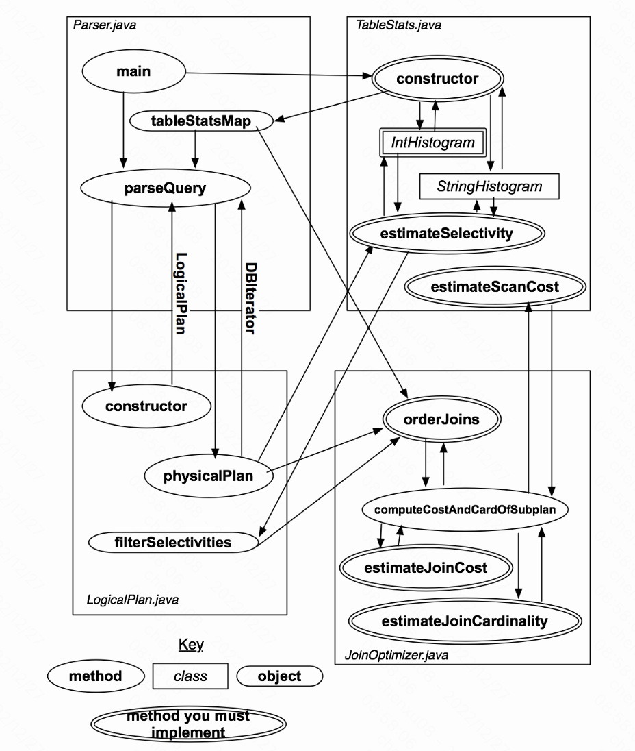
• Parser.java将会在初始化时构造一组表的统计信息，储存在statsMap中，等待query的输入后，则会调用parseQuery方法，转化query。
• parseQuery首先构造一个表示已解析查询的LogicalPlan。parseQuery然后在其已构造的LogicalPlan实例上调用physicalPlan方法。physicalPlan方法返回可用于实际运行查询的DBIterator对象。

---

二、实验过程

成本估算（Cost Estimation）：

成本估算（开销估算）是数据库系统评价一个访问计划优化好坏的标准。对于每一个生成的访问计划，优化器都必须根据相关统计信息（statistics）对其成本进行评估。

成本估算的主要指标是CPU时间和I/O数量。另外计算内存也是一个重要指标，不过这个指标的各个参数在数据库系统初始化时已经设定完成了，优化器并不能对这种硬性参数产生什么影响。所以可以将成本简化为CPU成本+I/O成本。
上一个成本估算的图：

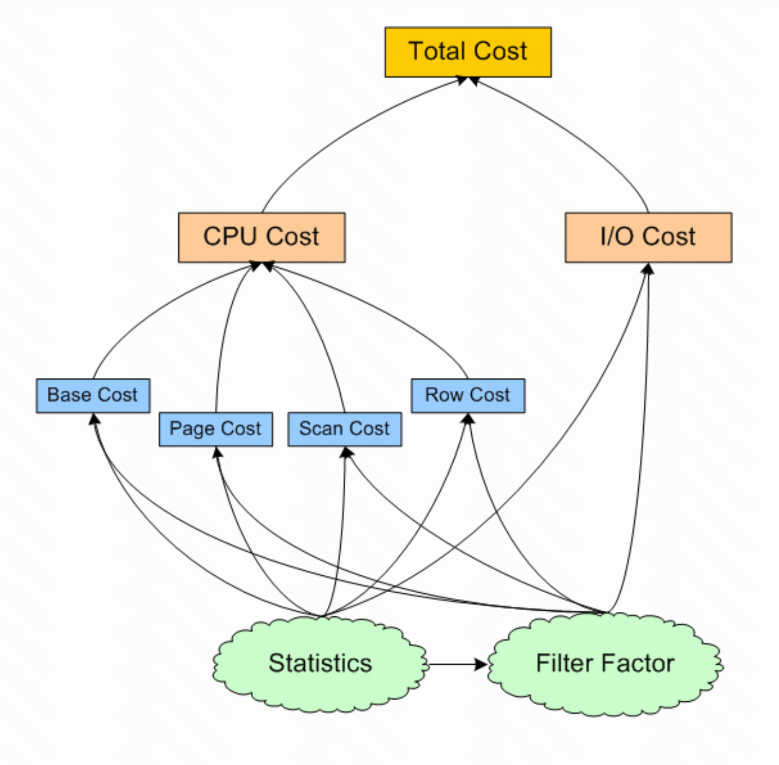
• I/O Cost:
  I/O成本指从磁盘取一页数据（一次I/O取一页数据）所花费的时间,一次I/O操作的经验时间是1/80秒。
• CPU Base Cost
  CPU基本成本指不依赖对象大小的一个值固定的CPU时间开销。
• CPU Page Cost
  CPU页成本指CPU从缓冲池中定位一个数据页的时间开销。
• CPU Scan Cost
  CPU扫描成本指对数据页中的记录（数据行）进行Sargable谓词扫描所需的时间开销。
• Sargable谓词
  考虑下面的SQL查询语句：
  Select * From EMPLOYEE Where EMPNO = 100 And DEPTNO <> 010
  Where条件子句后面的表达式EMPNO=100和DEPTNO<>010就是谓词，=、<>是操作符。所有的SQL谓词中，有些是可以使用索引的，有些则不能，例如在EMPNO和DEPTNO上分别创建了索引，EMPNO=100就可以利用EMPNO的索引优化查询，而DEPTNO<>010就无法使用DEPTNO上的索引了。
  IBM就将那些使用了诸如=,>,<,in,like等操作符的可以转化为索引操作的谓词称为Sargable谓词（Sargable是一个自创词，字典中是没有的）。可以译作可索引谓词。
  所以CPU Scan Cost可以理解成在数据页中使用可索引谓词来查找符合条件的记录（数据行）的时间开销。
• CPU Row Cost
  CPU行成本指将数据页中查找到的满足Sargable谓词条件的记录（数据行）复制到线程私有的内存空间以及对这些记录使用不可索引谓词进行进一步筛选所需的时间开销。
  该处使用的url网络请求的数据。

回到lab中的成本估计只关注表的连接成本和访问成本。不去考虑访问方法（Lab中只使用了一种访问方法，表扫描）和额外操作符（如聚合操作符）的成本。

而理解lab中的成本与直方图，还有两个重要的概念：基数和选择率。

基数和选择率

• 基数（cardinality)：一般情况下，某一列中，不同唯一键的数量。
  如果是主键列，每一行的键都是唯一存在的key，则主键的行数就是该列的基数。或者在一个一万行的性别列中，其取值，只有男、女，则该列的基数为2.
• 选择性(selectivity): 选择性 = 基数 / 行数。
  主键列选择性：1； 上述说的case则为：2 / 10000 = 0.0002 ；

基数选择性的作用：

• 列的选择性可以衡量数据库索引能够帮助缩小对表中特定值的搜索范围的程度。
  而我们知道索引最重要的目的之一是尽可能地缩小匹配行的初始候选值，从而减少io，提升查询性能。所以通常来说索引的选择性越高则查询效率越高，因为选择性高的索引可以让数据库在查找时过滤掉更多的行。
• CBO通常用选择率来估算对应结果集的基数。

回到lab中获每个字段的选择率，则是通过为每个字段建立一个直方图。

Exercise 1: IntHistogram

• 首先先全表扫描一次，获取每个字段的最大值与最小值。（目的是为了获得区间范围）。
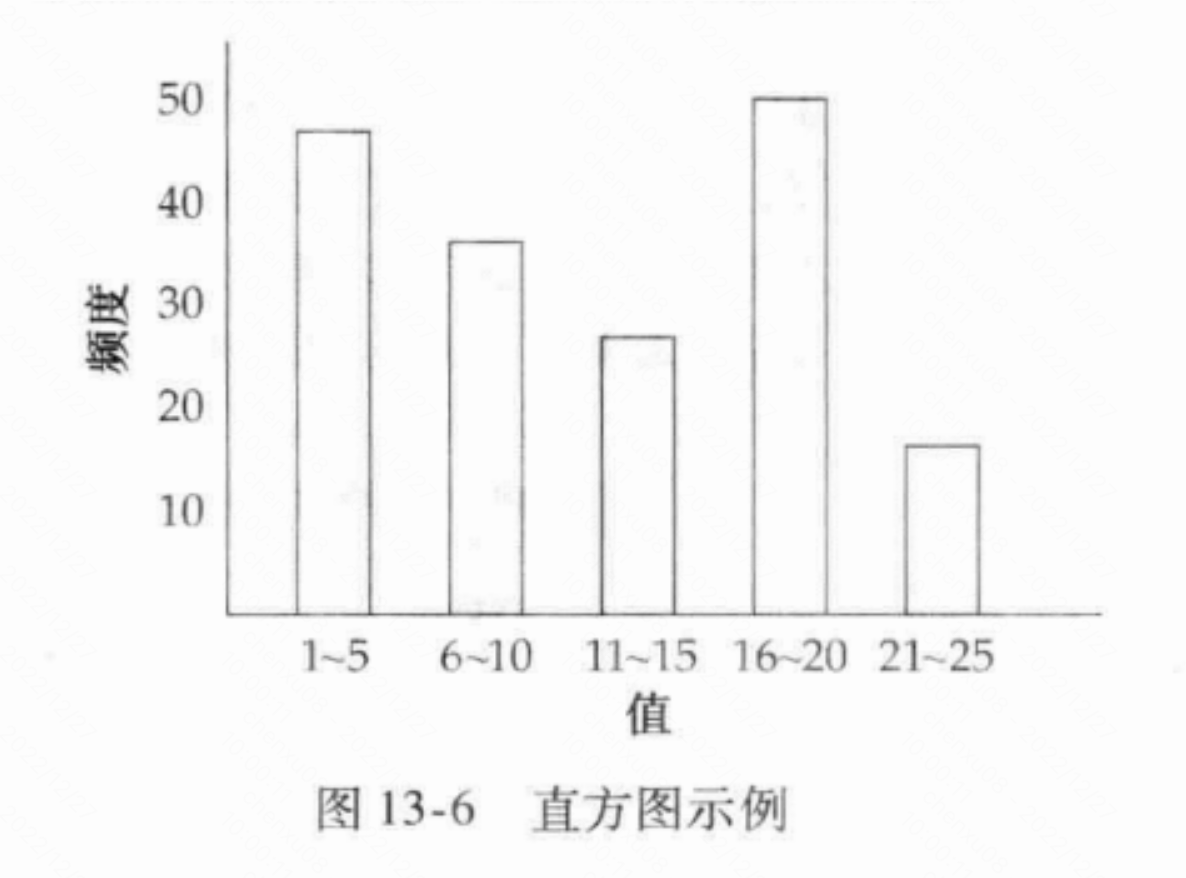
• 此时就可以建立直方图的初始坐标轴了，一种简单的方法是使用固定数量的桶NumB，每个桶表示直方图属性域的固定范围内的记录数。例如，如果字段f的范围从1到100，并且有10个存储桶，那么存储桶1可能包含1到10之间的记录数计数，存储桶2可能包含11到20之间的记录计数，依此类推。如：
  
• 再次扫描表，选择所有元组的所有字段，并使用它们填充每个直方图中的桶计数。

此时对于选择率则可以进行粗略的计算了：

• 对于等值运算value = const，首先需要找到包含该const值的桶，然后进行计算：选择率 = （value = const 的记录数）/ 记录总数，假设数值在桶中是均匀分布的，value = const的记录数为:( 桶高 / 桶宽)，故选择率可以表示为 （桶高 / 桶宽）/ 记录总数。
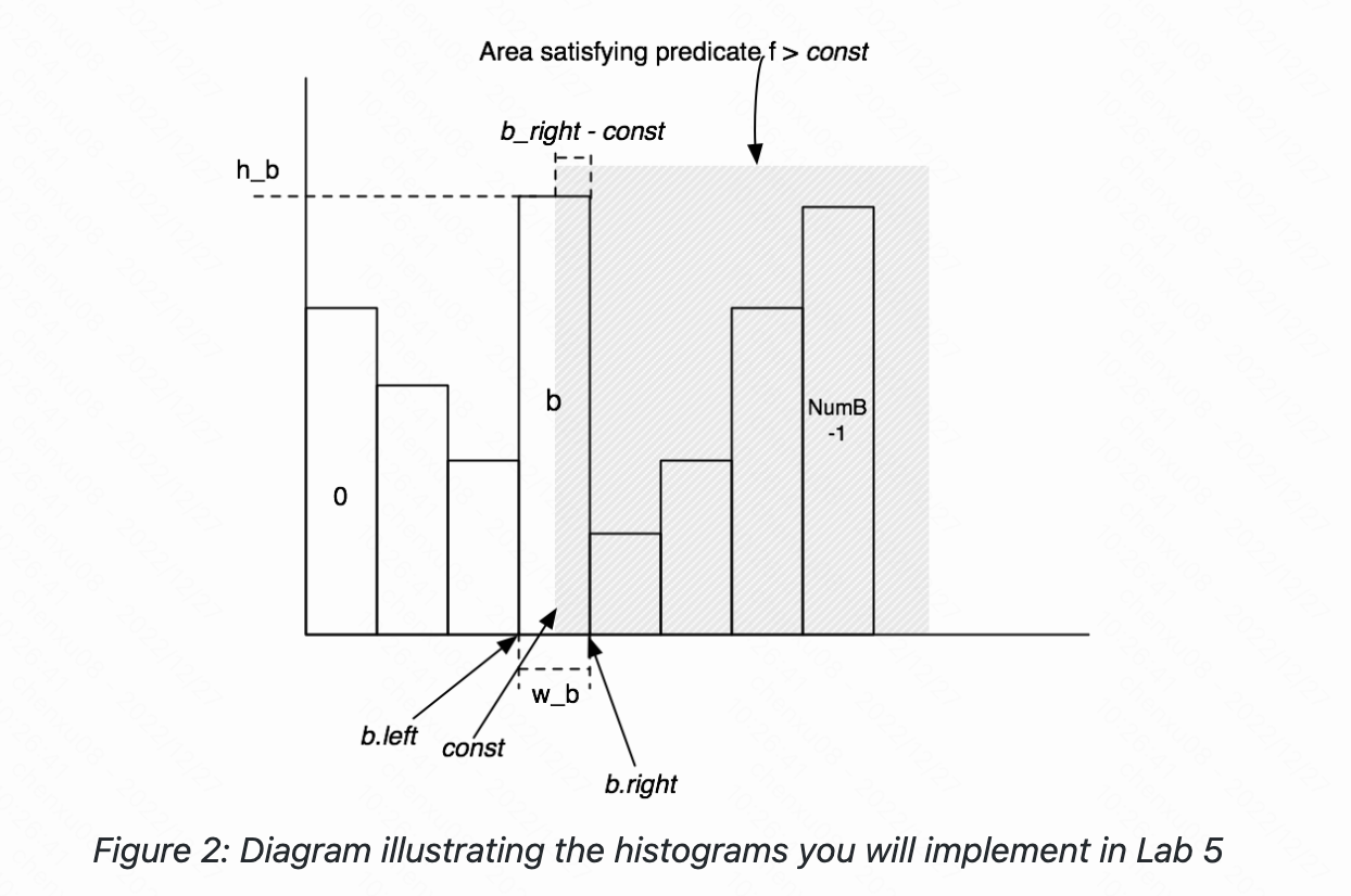
• 对于非等值运算，我们采用的也是同样的思想，value > const的选择率 = （value > const的记录数）/ 记录总数，value > const的记录数的记录数在直方图中由两部分构成。（const，b.right]部分的记录数 和 [b.right，max]部分的记录数。（const，b.right]部分的记录数 = （h_b / w_b）* （b_right - const）； [b.right，max]部分的记录数 = 后面桶高的加和。
  

• 在这里其实有个注意点：在桶数设置不合理的情况下，如1～25的情况下桶数设置的不为5，而是50，则桶宽则为0.5，而不是5。这个时候算选择性的时候则会变得更大，假如在0.5区间的数只有50，而除以0.5则变成100，而平均法下来的数据应该是只少不多，因此这是不合理的。此时就应该有两个修正方式：
• 在数据误差允许的范围内，将桶宽变为1，也就是进行一个Math.max(1,(1+Max-Min)/bucketLen)。
• 在每个字段的直方图选择性对比时，最后每个直方图设计的出来桶宽都要趋近相等。这样算出来的都是大的，则每个字段互相对比就影响不大，而对于同款趋近相等则应该不断维护一个最小桶宽数，然后每次最小桶宽数（width < 1)更新时应该同步更改别的直方图的桶数，最后使每个直方图的桶宽趋近一致。但这在大宽表时，效率则会变很低。 且选择性从几何角度上来说，应该是要小于1的，因为假设传入的非等值操作为v > max,则获取的数据应该为ntups（元组总数）/ntups = 1，也就是占了直方图面积的百分百。

而回归本次lab，应该选取第一种计算方法，也就是Math.max(1,(1+Max-Min)/bucketLen)。 因为测试数据都是给定的。

• IntHistogram Class:

public class IntHistogram {

    private int[] buckets;
    private int min;
    private int max;
    private double width;

    /**
     * 元组记录总数
     */
    private int ntups;

    /**
     * Create a new IntHistogram.
     * <p>
     * This IntHistogram should maintain a histogram of integer values that it receives.
     * It should split the histogram into "buckets" buckets.
     * <p>
     * The values that are being histogrammed will be provided one-at-a-time through the "addValue()" function.
     * <p>
     * Your implementation should use space and have execution time that are both
     * constant with respect to the number of values being histogrammed.  For example, you shouldn't
     * simply store every value that you see in a sorted list.
     *
     * @param buckets The number of buckets to split the input value into.
     * @param min     The minimum integer value that will ever be passed to this class for histogramming
     * @param max     The maximum integer value that will ever be passed to this class for histogramming
     */
    public IntHistogram(int buckets, int min, int max) {
        // some code goes here
        this.buckets = new int[buckets];
        this.min = min;
        this.max = max;
        this.width = Math.max(1,(max - min + 1.0) / buckets);
        this.ntups = 0;
    }

    /**
     * Add a value to the set of values that you are keeping a histogram of.
     *
     * @param v Value to add to the histogram
     */
    public void addValue(int v) {
        // some code goes here
        if(v >= min && v <= max && getIndex(v) != -1){
            buckets[getIndex(v)]++;
            ntups++;
        }
    }

    public int getIndex(int v){
        int index = (int) ((v - min) / width);
        if(index < 0 || index >= buckets.length){
            return -1;
        }
        return index;
    }

    /**
     * Estimate the selectivity of a particular predicate and operand on this table.
     * <p>
     * For example, if "op" is "GREATER_THAN" and "v" is 5,
     * return your estimate of the fraction of elements that are greater than 5.
     *
     * @param op Operator
     * @param v  Value
     * @return Predicted selectivity of this particular operator and value
     */
    public double estimateSelectivity(Predicate.Op op, int v) {

        // some code goes here
        // case: 2、3、4、5； 6，7，8，9； v = 7
        switch(op){

            // 8，9
            case GREATER_THAN:
                if(v > max){
                    return 0.0;
                } else if (v <= min){
                    return 1.0;
                } else {
                    int index = getIndex(v);
                    double tuples = 0;
                    for(int i = index + 1; i < buckets.length; i++){
                        tuples += buckets[i];
                    }
                    // 2 * 4 + 2 - 1 -7
                    tuples += (min + (getIndex(v) + 1) * width - 1 - v) *  (1.0 *buckets[index] / width);
                    return tuples / ntups;
                }
            case LESS_THAN:
                return 1 - estimateSelectivity(Predicate.Op.GREATER_THAN_OR_EQ,v);
            case EQUALS:
                return estimateSelectivity(Predicate.Op.LESS_THAN_OR_EQ, v) -
                        estimateSelectivity(Predicate.Op.LESS_THAN, v);
            case NOT_EQUALS:
                return 1 - estimateSelectivity(Predicate.Op.EQUALS,v);
            case GREATER_THAN_OR_EQ:
                return estimateSelectivity(Predicate.Op.GREATER_THAN,v-1);
            case LESS_THAN_OR_EQ:
                return estimateSelectivity(Predicate.Op.LESS_THAN,v+1);
            default:
                throw new UnsupportedOperationException("Op is illegal");
        }
    }

    /**
     * @return the average selectivity of this histogram.
     *         <p>
     *         This is not an indispensable method to implement the basic
     *         join optimization. It may be needed if you want to
     *         implement a more efficient optimization
     */
    public double avgSelectivity() {
        // some code goes here
        double sum = 0;
        for (int bucket : buckets) {
            sum += (1.0 * bucket / ntups);
        }
        return sum / buckets.length;
    }

    /**
     * @return A string describing this histogram, for debugging purposes
     */
    public String toString() {
        // some code goes here
        return "IntHistogram{" +
                "buckets = " + Arrays.toString(buckets) +
                ", min = " + min +
                ", max =" + max +
                ", width =" + width +
                "}";
    }
}

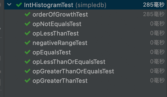
• 测试结果：
  

---

Exercise 2: TableStats

对于Exercise 2，主要是完成TableStats类，传入tableId，与每页的IO花销，构造每个字段的直方图，并利用Exercise1的方法，得出每个直方图相关的选择性估算。

• TableStats Class:

public class TableStats {

    private static final ConcurrentMap<String, TableStats> statsMap = new ConcurrentHashMap<>();

    static final int IOCOSTPERPAGE = 1000;

    /**
     * Number of bins for the histogram. Feel free to increase this value over
     * 100, though our tests assume that you have at least 100 bins in your
     * histograms.
     */
    static final int NUM_HIST_BINS = 100;

    private int ioCostPerPage;

    private ConcurrentHashMap<Integer, IntHistogram> intHistograms;

    private ConcurrentHashMap<Integer, StringHistogram> strHistograms;
    private  HeapFile dbFile;
    private TupleDesc td;
    /**
     * 传入表的总记录数，用于估算estimateTableCardinality
     */
    private int totalTuples;



    public static TableStats getTableStats(String tablename) {
        return statsMap.get(tablename);
    }

    public static void setTableStats(String tablename, TableStats stats) {
        statsMap.put(tablename, stats);
    }

    public static void setStatsMap(Map<String, TableStats> s) {
        try {
            java.lang.reflect.Field statsMapF = TableStats.class.getDeclaredField("statsMap");
            statsMapF.setAccessible(true);
            statsMapF.set(null, s);
        } catch (NoSuchFieldException | IllegalAccessException | IllegalArgumentException | SecurityException e) {
            e.printStackTrace();
        }

    }

    public static Map<String, TableStats> getStatsMap() {
        return statsMap;
    }

    public static void computeStatistics() {
        Iterator<Integer> tableIt = Database.getCatalog().tableIdIterator();

        System.out.println("Computing table stats.");
        while (tableIt.hasNext()) {
            int tableid = tableIt.next();
            TableStats s = new TableStats(tableid, IOCOSTPERPAGE);
            setTableStats(Database.getCatalog().getTableName(tableid), s);
        }
        System.out.println("Done.");
    }



    /**
     * Create a new TableStats object, that keeps track of statistics on each
     * column of a table
     *
     * @param tableid       The table over which to compute statistics
     * @param ioCostPerPage The cost per page of IO. This doesn't differentiate between
     *                      sequential-scan IO and disk seeks.
     */
    public TableStats(int tableid, int ioCostPerPage) {
        // For this function, you'll have to get the
        // DbFile for the table in question,
        // then scan through its tuples and calculate
        // the values that you need.
        // You should try to do this reasonably efficiently, but you don't
        // necessarily have to (for example) do everything
        // in a single scan of the table.
        // some code goes here
        Map<Integer, Integer> minMap = new HashMap<>();
        Map<Integer, Integer> maxMap = new HashMap<>();
        this.intHistograms = new ConcurrentHashMap<>();
        this.strHistograms = new ConcurrentHashMap<>();
        this.dbFile = (HeapFile)Database.getCatalog().getDatabaseFile(tableid);
        this.ioCostPerPage = ioCostPerPage;
        this.td = dbFile.getTupleDesc();

        Transaction tx = new Transaction();
        tx.start();
        DbFileIterator child = dbFile.iterator(tx.getId());

        try {
            child.open();
            while (child.hasNext()) {
                this.totalTuples++;
                Tuple tuple = child.next();
                for (int i = 0; i < td.numFields(); i++) {
                    if (td.getFieldType(i).equals(Type.INT_TYPE)) {
                        //Int类型，需要先统计各个属性的最大最小值
                        IntField field = (IntField) tuple.getField(i);
                        //最小值
                        minMap.put(i, Math.min(minMap.getOrDefault(i, Integer.MAX_VALUE), field.getValue()));
                        //最大值
                        maxMap.put(i, Math.max(maxMap.getOrDefault(i, Integer.MIN_VALUE), field.getValue()));
                    } else if(td.getFieldType(i).equals(Type.STRING_TYPE)){
                        StringHistogram histogram = this.strHistograms.getOrDefault(i, new StringHistogram(NUM_HIST_BINS));
                        StringField field = (StringField) tuple.getField(i);
                        histogram.addValue(field.getValue());
                        this.strHistograms.put(i, histogram);
                    }
                }
            }
            // 根据最大最小值构造直方图
            for (int i = 0; i < td.numFields(); i++) {
                if (minMap.get(i) != null) {
                    //初始化构造int型直方图
                    this.intHistograms.put(i, new IntHistogram(NUM_HIST_BINS, minMap.get(i), maxMap.get(i)));
                }
            }
            // 重新扫描表，往Int直方图添加数据
            child.rewind();
            while (child.hasNext()) {
                Tuple tuple = child.next();
                //填充直方图的数据
                for (int i = 0; i < td.numFields(); i++) {
                    if (td.getFieldType(i).equals(Type.INT_TYPE)) {
                        IntField f = (IntField) tuple.getField(i);
                        IntHistogram intHis = this.intHistograms.get(i);
                        if (intHis == null) throw new IllegalArgumentException("获得直方图失败！！");
                        intHis.addValue(f.getValue());
                        this.intHistograms.put(i, intHis);
                    }
                }
            }
        } catch (Exception e) {
            e.printStackTrace();
        }finally {
            child.close();
            try {
                tx.commit();
            } catch (IOException e) {
                System.out.println("事务提交失败！！");
            }

        }

    }

    /**
     * Estimates the cost of sequentially scanning the file, given that the cost
     * to read a page is costPerPageIO. You can assume that there are no seeks
     * and that no pages are in the buffer pool.
     * <p>
     * Also, assume that your hard drive can only read entire pages at once, so
     * if the last page of the table only has one tuple on it, it's just as
     * expensive to read as a full page. (Most real hard drives can't
     * efficiently address regions smaller than a page at a time.)
     *
     * @return The estimated cost of scanning the table.
     */
    public double estimateScanCost() {
        // some code goes here
        // 文件所需的页数 * IO单次花费 * 遍历的轮次
        return dbFile.numPages() * ioCostPerPage * 2;
    }

    /**
     * This method returns the number of tuples in the relation, given that a
     * predicate with selectivity selectivityFactor is applied.
     *
     * @param selectivityFactor The selectivity of any predicates over the table
     * @return The estimated cardinality of the scan with the specified
     *         selectivityFactor
     */
    public int estimateTableCardinality(double selectivityFactor) {
        // some code goes here
        return (int) ( totalTuples * selectivityFactor);
    }

    /**
     * The average selectivity of the field under op.
     *
     * @param field the index of the field
     * @param op    the operator in the predicate
     *              The semantic of the method is that, given the table, and then given a
     *              tuple, of which we do not know the value of the field, return the
     *              expected selectivity. You may estimate this value from the histograms.
     */
    public double avgSelectivity(int field, Predicate.Op op) {
        // some code goes here
        if (td.getFieldType(field).equals(Type.INT_TYPE)) {
            return intHistograms.get(field).avgSelectivity();
        }else if(td.getFieldType(field).equals(Type.STRING_TYPE)){
            return strHistograms.get(field).avgSelectivity();
        }
        return -1.00;
    }

    /**
     * Estimate the selectivity of predicate <tt>field op constant</tt> on the
     * table.
     *
     * @param field    The field over which the predicate ranges
     * @param op       The logical operation in the predicate
     * @param constant The value against which the field is compared
     * @return The estimated selectivity (fraction of tuples that satisfy) the
     *         predicate
     */
    public double estimateSelectivity(int field, Predicate.Op op, Field constant) {
        // some code goes here
        if (td.getFieldType(field).equals(Type.INT_TYPE)) {
            IntField intField = (IntField) constant;
            return intHistograms.get(field).estimateSelectivity(op,intField.getValue());
        } else if(td.getFieldType(field).equals(Type.STRING_TYPE)){
            StringField stringField = (StringField) constant;
            return strHistograms.get(field).estimateSelectivity(op,stringField.getValue());
        }
        return -1.00;
    }

    /**
     * return the total number of tuples in this table
     */
    public int totalTuples() {
        // some code goes here
        return totalTuples;
    }

}

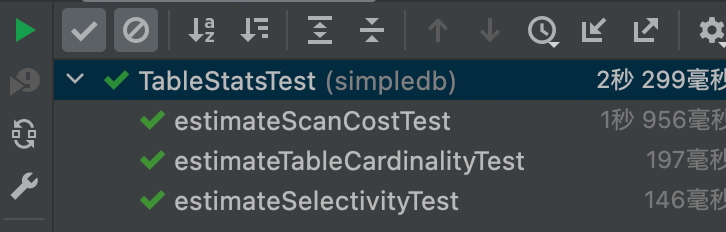
• 测试结果：
  

---

Exercise 3: Join Cost Estimation

对于Exercise3则是进行对连接成本的估算，回到lab中对join成本估算的公式：

joincost(t1 join t2) = scancost(t1) + ntups(t1) x scancost(t2) //IO cost + ntups(t1) x ntups(t2) //CPU cost

拿笔者上一篇的case举例下：
-假设目前有一个join操作：对两个chidren中的sex字段进行自然连接。

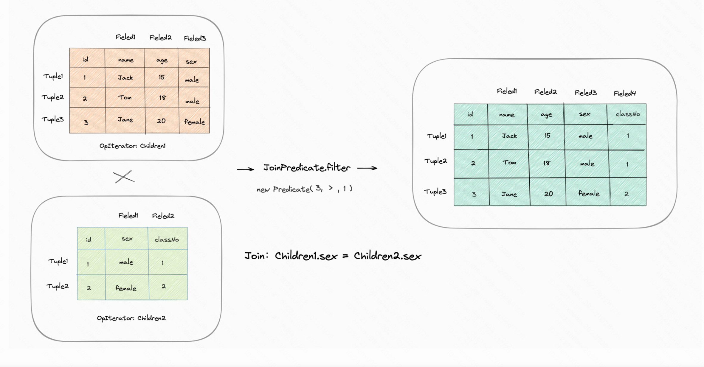
则首先需要从磁盘中获取children1中的记录则此部分的开销为scancost(t1), 而后children1中的每一条记录都需要遍历children2中哪条数据符合而这记录的开销为ntups(t1) x scancost(t2) 。而这整体下来的操作在代码中的实现为双重循环，也就是CPU的开销应该为ntups(t1) x ntups(t2)。

public double estimateJoinCost(LogicalJoinNode j, int card1, int card2,
                                   double cost1, double cost2) {
        if (j instanceof LogicalSubplanJoinNode) {
            // A LogicalSubplanJoinNode represents a subquery.
            // You do not need to implement proper support for these for Lab 3.
            return card1 + cost1 + cost2;
        } else {
            // Insert your code here.
            // HINT: You may need to use the variable "j" if you implemented
            // a join algorithm that's more complicated than a basic
            // nested-loops join.
            return cost1 + card1 * cost2 + card1 * card2;
        }
    }

而对于基数的估计根据lab应该注意以下几点：

• 对于相等联接，当其中一个属性是主键时，联接产生的元组数不能大于非主键属性的基数。
• 对于没有主键的相等联接，很难说输出的大小是多少——它可以是表的基数的乘积的大小（如果两个表对于所有元组都具有相同的值）——或者可以是0。制定一个简单的启发式方法（比如两个表中较大的表的大小）是很好的。
• 对于范围扫描，同样很难估计出其连接的大小。输出的大小应与输入的大小成正比，通常选用连接的两个基数的交叉积的30%。

在这里其实可以思考下基数的本质是为了什么，是为了估计选择性，大多数的时候就是为了判断这个字段是否更适合索引，也就是数据采样是否更具特异性。 如果这个选择性，接近0，说明其的采样范围少，重复的数据多。而接近1则是说明其采样范围多，重复数据少。而自然连接本质其实就是取两个集合根据特定条件而连接的交集。 因此通过这两点反过来回去想以上几点就很好理解了：

• 对与有主键的连接中，应该选取非主键的基数。因为主键的基数很大，而非主键的基数很小，那么连接后的结果中采样范围更具特异性的应该是非主键的。
• 如果两者都是主键的，那么应该取更小范围的，会更具特异性。
• 如果都是非主键的，则通过hint中的，取更大的。

	/**
     * Estimate the join cardinality of two tables.
     */
    public static int estimateTableJoinCardinality(Predicate.Op joinOp,
                                                   String table1Alias, String table2Alias, String field1PureName,
                                                   String field2PureName, int card1, int card2, boolean t1pkey,
                                                   boolean t2pkey, Map<String, TableStats> stats,
                                                   Map<String, Integer> tableAliasToId) {
        int card = 1;
        // some code goes here
        if(joinOp == Predicate.Op.EQUALS){
            if (t1pkey && !t2pkey) {
                card = card2;
            } else if (!t1pkey && t2pkey) {
                card = card1;
            } else if (t1pkey && t2pkey) {
                card = Math.min(card1, card2);
            } else {
                card = Math.max(card1, card2);
            }
        } else {
            card = (int) (0.3 * card1 * card2);
        }
        return card <= 0 ? 1 : card;
    }

---

Exercise 4: Join Cost Estimation

对于Exercise4则是总体生成优化过后的连接顺序。根据上述提供的计算成本的公式，不同顺序的连接成本也不同。在《数据库系统概念》书中是这样描述的：

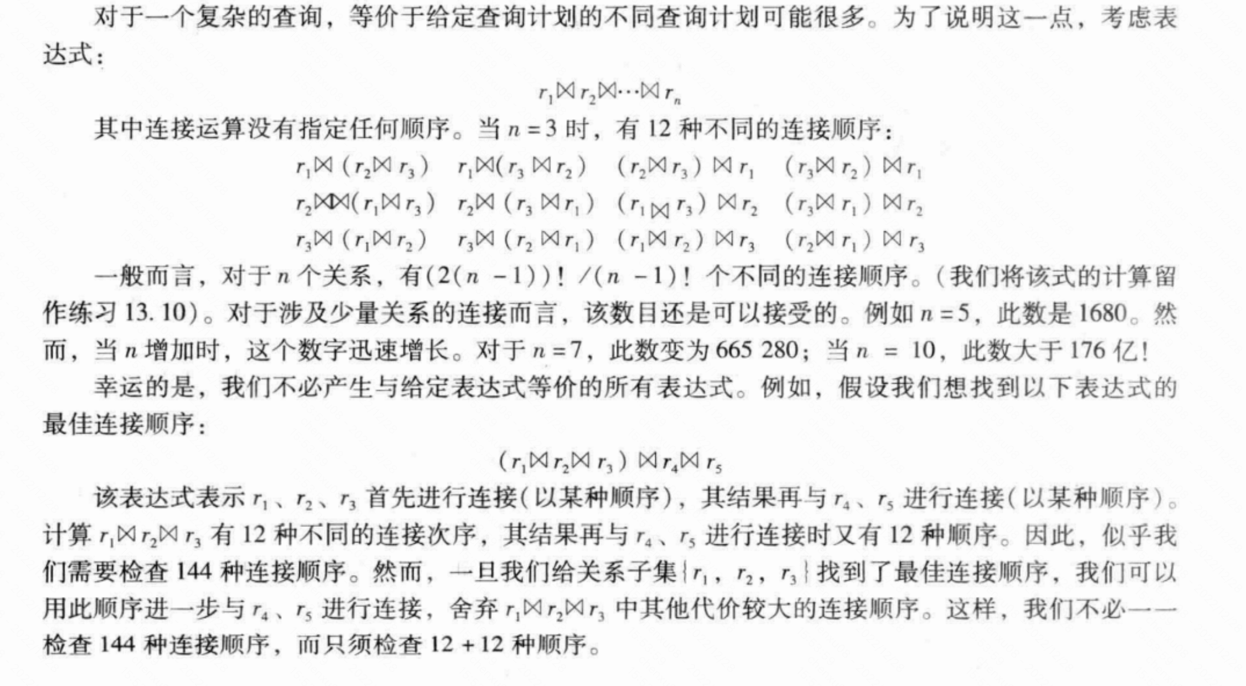
由此思想而给出的动态规划的伪代码：

produe FindBestPlan(S)
	if(bestplan[S].cost ≠ ∞ ) 	//bestplan[S]已经计算好了
		return bestplan[S]
	if(S中只包含一个关系)
		根据访问S的最佳方式设置bestplan[S].plan和bestplab[S].cost
	else
		for each S 的非空子集S1，且S1≠S
			P1 = FindBestPlan(S1)
			P2 = FindBestPlan(S-S1)
			A = 连接P1和P2的结果的算法   //嵌套循环连接
			plan = 使用A对P1和P2进行连接的结果
			cost = P1.cost + P2.cost + A的代价
			if  cost < bestplan[S].cost
				bestplan[S].cost = cost
				bestplan[S].plan = plan
return bestplan[S]

对于lab还提供了几个辅助类与方法：

• CostCard:由计划表示的最优计划的成本和基数。
• PlanCache:助手类，可用于存储最好的连接集排序的方法。
• enumerateSubsets(List<T> v, int size) :生成给定大小的子集合。
• CostCard computeCostAndCardOfSubplan()：计算子计划的查询代价。
• printJoins：将连接计划进行特定格式打印。

    public List<LogicalJoinNode> orderJoins(
            Map<String, TableStats> stats,
            Map<String, Double> filterSelectivities, boolean explain)
            throws ParsingException {
        // Not necessary for labs 1 and 2.

        // some code goes here
        CostCard bestCostCard = new CostCard();
        PlanCache planCache = new PlanCache();
        // 思路：通过辅助方法获取每个size下最优的连接顺序，不断加入planCache中
        for (int i = 1; i <= joins.size(); i++) {
            Set<Set<LogicalJoinNode>> subsets = enumerateSubsets(joins, i);
            for (Set<LogicalJoinNode> set : subsets) {
                double bestCostSoFar = Double.MAX_VALUE;
                bestCostCard = new CostCard();
                for (LogicalJoinNode logicalJoinNode : set) {
                    //根据子计划找出最优的方案
                    CostCard costCard = computeCostAndCardOfSubplan(stats, filterSelectivities, logicalJoinNode, set, bestCostSoFar, planCache);
                    if (costCard == null) continue;
                    bestCostSoFar = costCard.cost;
                    bestCostCard = costCard;
                }
                if (bestCostSoFar != Double.MAX_VALUE) {
                    planCache.addPlan(set, bestCostCard.cost, bestCostCard.card, bestCostCard.plan);
                }
            }
        }
        if (explain){
            printJoins(bestCostCard.plan, planCache, stats, filterSelectivities);
        }

        // 如果joins传进来的长度为0，则计划就为空
        if(bestCostCard.plan != null){
            return bestCostCard.plan;
        }
        return joins;
    }

• 测试结果：
  
  

---

Extra Credit

主要对enumerateSubsets进行优化：

• Improved subset iterator. Our implementation of enumerateSubsets() is quite inefficient, because it creates a large number of Java objects on each invocation. In this bonus exercise, you would improve the performance of enumerateSubsets() so that your system could perform query optimization on plans with 20 or more joins (currently such plans takes minutes or hours to compute)。

对于全排列，最好的优化方式应该是回溯+减枝，否则对于本lab的优化时间则差不多。

• 时间复杂度：k * n!，其中k为size的大小。
• 空间复杂度：空间复杂度：O(n)其中 n 为列表的长度。除答案数组以外，递归函数在递归过程中需要为每一层递归函数分配栈空间，所以这里需要额外的空间且该空间取决于递归的深度，这里可知递归调用深度为 O(n)。

public <T> Set<Set<T>> enumerateSubsets(List<T> v, int size) {
        Set<Set<T>> els = new HashSet<>();
        dfs(els,v ,size, 0, new LinkedList<>());
        return els;

    }
    private <T> void dfs(Set<Set<T>> els, List<T> v, int size, int curIdx, Deque<T> path) {
        if (path.size() == size) {
            els.add(new HashSet<>(path));
            return;
        }
        if (curIdx == size) {
            return;
        }
        path.addFirst(v.get(curIdx));
        dfs(els, v, size, curIdx + 1, path);
        path.removeFirst();
        dfs(els, v, size, curIdx + 1, path);
    }

会快一些，主要看剪枝的效率：

---

总结

对于此次的lab相较于上一次，理解难度会高一些，需要理解基数，选择性等概念，而理解后实际编写难度可能会低一些。在此次lab中比较花时间的其实还有queryTest的跑通，有些逻辑要根据测试的逻辑来编写，例如表的别名那里，否则会报一系列错误。此次的lab在工作之余大概断断续续写了两天，到这6.830也完成一半了，剩下的会在明年初陆陆续续的赶完。如有不足欢迎指正～