RegNet的博客的准备我可谓是话费了很多的时间,参考了诸多大佬的资料,主要是网上对于这个网络的讲解有点少,毕竟这个网络很新。网上可以参考的资料太少,耗费了相当多的时间,不过一切都是值得的,毕竟学完之后,才发现它真的是个超级无敌吊炸天的CNN卷积神经网络,跟他比起来之前常规的神经网络完全都是弟弟!好的 废话少说,我们先来简单了解一下regnet的思想。
原论文名称:Designing Network Design Spaces
原论文下载地址:https://arxiv.org/abs/2003.13678.pdf
论文中提供的源码: https://github.com/facebookresearch/pycls
自己使用网上大佬们的代码魔改的,RegNet代码(Pytorch实现):
链接:https://pan.baidu.com/s/13J06nZimdZacCP20js0mUg
提取码:oyc3
学习Regnet的时候网上一顿搜,然后都出来什么搜索空间等等一大堆,看的我贼懵逼,让我难受了半天,一直无法得到Regnet的核心思想,类似Resnet的残差思想,Densnet的密接思想,直到我看到了这位B站大佬的短短十几分钟简单的讲述我才明白什么叫做Regnet。
这里链接给出:自动驾驶系列论文解读(一):RegNet——颠覆NAS的AutoML文章_哔哩哔哩_bilibili
如果不愿意看视频的话,请听鄙人简单概括通俗易懂的讲述一下!
我认为Regnet的出现是具有颠覆性的,正如人们学习的过程那样,都是从微观到宏观,Regnet从更宏观的角度看待神经网络,让之前的NAS搜索算法看起来像个笑话。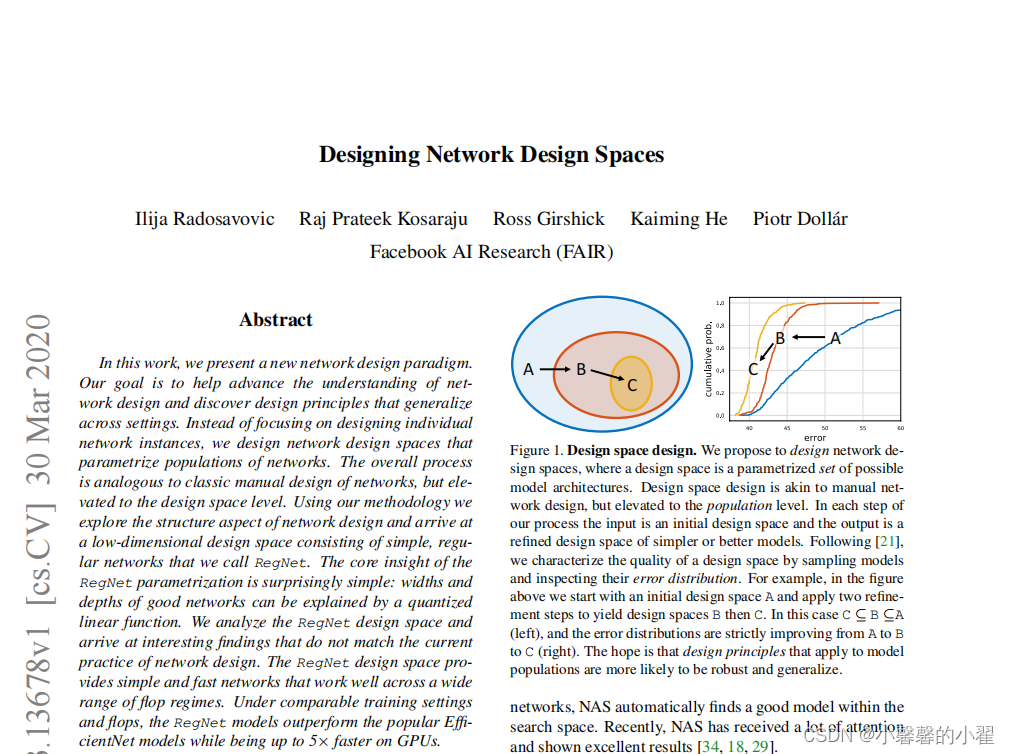
首先学习这个的时候,我希望我们是有一些CNN的基础,类似Alexnet和Resnet都是懂的,这样我们才能比较快的学到这个。好的 我们开始讲。
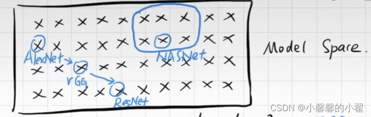
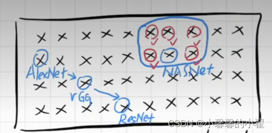
正如上图所示,我们可以想象一下我们所有的网络结构组成一个空间,那我们之前学过的例如Alexnet,VGG,Resnet都是空间中的某个点,这都是人类发展过程中寻找的比较好的网络结构,但是随着人类的发展,人们日益增长的需求发现之前的网络结构一定不是最优的最好的,这个空间内肯定存在很多好的网络结构,这也是我们发展的过程,但是这和个空间很庞大,优秀的网络结构如果靠人们一个一个去试的话未免是不是有些太费劲了。
就在这个时候出现了NASnet,搜索神经网络,
NASnet,搜索神经网络:
所谓搜索神经网络,就是人们手动划分一个这个空间的子空间,然后使用搜索的办法去寻找最优解,但是事实上这个方法依然是落后的,第一NAS系列的算法跑起来贼TM费算力和时间,即便是最优秀的显卡也需要跑很长时间。这是个非常大的弊端。其次:如上图所示,就算我们找到了一个最优解(蓝色的)。
第一:
如果说他周围的临近点(所谓点,就是表现好的神经网络架构) 表现也不好的话,那我们不得不怀疑这个表现好的点(蓝色)其实效果应该也没有那么好,只不过是因为适应了当前这个数据集,从而导致有些过拟合的风险。
第二:
如果他周围的临近点表现也好的话,那这个就更没意义了,既然都表现好,那是不是说明人工选择的这个子空间好呢?这样NAS的优秀难道不是依赖于人工子空间的选择吗?
以上两个问题让NAS搜索系列神经网络看起来像个笑话。
Regnet的核心思想在于如何去设计一个有效的空间,并发现一些网络的通用设计准则,然后根据相应数据集,自动找到最优的参数。当然我们会设定一个范围。
简单来说就是如何设计一个有效的方法,找到有效的空间去搜索我们需要的参数,对就是这样,不再人工选择空间搜索,而是找到一个寻找空间的方法,去搜索最优的参数。
这就是超级无敌吊炸天的Regnet。当然这只是个思想,具体的细节我们还是要读论文才知道。
好的,下面我们看一下Regnet的网络结构
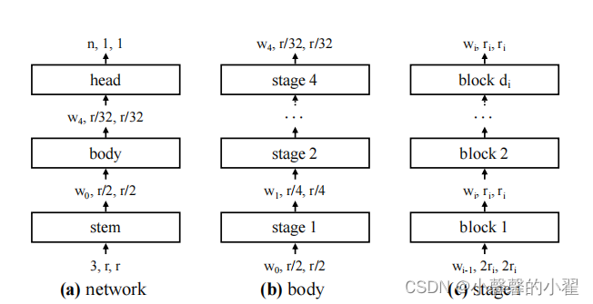
Regnet网络主要由三部分组成,stem、body和head。
其中stem就是一个普通的卷积层(默认包含BN以及激活函数RELU),卷积核大小为3x3,步距为2,卷积核个数为32.
其中body就是由4个stage堆叠组成,如图(b)所示。每经过一个stage都会将输入特征矩阵的height和width缩减为原来的一半。而每个stage又是由一系列block堆叠组成,每个stage的第一个block中存在步距为2的组卷积(主分支上)和普通卷积(捷径分支上),剩下的block中的卷积步距都是1,和ResNet类似。
其中head就是分类网络中常见的分类器,由一个全局平均池化层和全连接层构成。
下面是BLOCK模板的结构图:
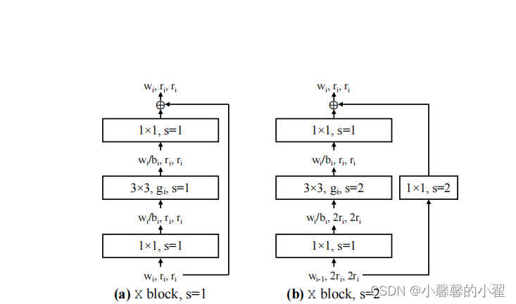
跟ResNet网络中的block基本一致。主分支都是一个1x1的卷积(包括BN以及激活函数RELU)、一个3x3的group卷积(包括BN以及激活函数RELU)、再接一个1x1的卷积(包括BN)。shortcut捷径分支上当stride=1时不做任何处理,当stride=2时通过一个1x1的卷积(包括BN)进行下采样。论文上的图不清楚,太乱,这里霹雳大佬换了新的,这里注明出处:
RegNet网络结构与搭建_太阳花的小绿豆的博客-CSDN博客_regnet网络结构

好的知道了网络结构,我们要开始发布我们的注释代码了,代码也是参考了霹雳大佬的和网上其他大佬的魔改了一下,改的可以生成训练集和测试集的准确率和损失,并且绘制相应1的折线图。
代码详解部分:
网络结构源代码部分:
from typing import Optional

import numpy as np
import torch
import torch.nn as nn
from torch import Tensor


def _make_divisible(ch, divisor=8, min_ch=None):
    """
    This function is taken from the original tf repo.
    It ensures that all layers have a channel number that is divisible by 8
    It can be seen here:
    https://github.com/tensorflow/models/blob/master/research/slim/nets/mobilenet/mobilenet.py
    """
    if min_ch is None:
        min_ch = divisor
    new_ch = max(min_ch, int(ch + divisor / 2) // divisor * divisor)
    # Make sure that round down does not go down by more than 10%.
    if new_ch < 0.9 * ch:
        new_ch += divisor
    return new_ch


def _mcfg(**kwargs):
    cfg = dict(se_ratio=0., bottle_ratio=1., stem_width=32)#请注意这里这个32,这个32就是stem里面的32个卷积核
    cfg.update(**kwargs)
    return cfg


model_cfgs = {
    "regnetx_200mf": _mcfg(w0=24, wa=36.44, wm=2.49, group_w=8, depth=13),
    "regnetx_400mf": _mcfg(w0=24, wa=24.48, wm=2.54, group_w=16, depth=22),
    "regnetx_600mf": _mcfg(w0=48, wa=36.97, wm=2.24, group_w=24, depth=16),
    "regnetx_800mf": _mcfg(w0=56, wa=35.73, wm=2.28, group_w=16, depth=16),
    "regnetx_1.6gf": _mcfg(w0=80, wa=34.01, wm=2.25, group_w=24, depth=18),
    "regnetx_3.2gf": _mcfg(w0=88, wa=26.31, wm=2.25, group_w=48, depth=25),
    "regnetx_4.0gf": _mcfg(w0=96, wa=38.65, wm=2.43, group_w=40, depth=23),
    "regnetx_6.4gf": _mcfg(w0=184, wa=60.83, wm=2.07, group_w=56, depth=17),
    "regnetx_8.0gf": _mcfg(w0=80, wa=49.56, wm=2.88, group_w=120, depth=23),
    "regnetx_12gf": _mcfg(w0=168, wa=73.36, wm=2.37, group_w=112, depth=19),
    "regnetx_16gf": _mcfg(w0=216, wa=55.59, wm=2.1, group_w=128, depth=22),
    "regnetx_32gf": _mcfg(w0=320, wa=69.86, wm=2.0, group_w=168, depth=23),
    "regnety_200mf": _mcfg(w0=24, wa=36.44, wm=2.49, group_w=8, depth=13, se_ratio=0.25),
    "regnety_400mf": _mcfg(w0=48, wa=27.89, wm=2.09, group_w=8, depth=16, se_ratio=0.25),
    "regnety_600mf": _mcfg(w0=48, wa=32.54, wm=2.32, group_w=16, depth=15, se_ratio=0.25),
    "regnety_800mf": _mcfg(w0=56, wa=38.84, wm=2.4, group_w=16, depth=14, se_ratio=0.25),
    "regnety_1.6gf": _mcfg(w0=48, wa=20.71, wm=2.65, group_w=24, depth=27, se_ratio=0.25),
    "regnety_3.2gf": _mcfg(w0=80, wa=42.63, wm=2.66, group_w=24, depth=21, se_ratio=0.25),
    "regnety_4.0gf": _mcfg(w0=96, wa=31.41, wm=2.24, group_w=64, depth=22, se_ratio=0.25),
    "regnety_6.4gf": _mcfg(w0=112, wa=33.22, wm=2.27, group_w=72, depth=25, se_ratio=0.25),
    "regnety_8.0gf": _mcfg(w0=192, wa=76.82, wm=2.19, group_w=56, depth=17, se_ratio=0.25),
    "regnety_12gf": _mcfg(w0=168, wa=73.36, wm=2.37, group_w=112, depth=19, se_ratio=0.25),
    "regnety_16gf": _mcfg(w0=200, wa=106.23, wm=2.48, group_w=112, depth=18, se_ratio=0.25),
    "regnety_32gf": _mcfg(w0=232, wa=115.89, wm=2.53, group_w=232, depth=20, se_ratio=0.25)
}


def generate_width_depth(wa, w0, wm, depth, q=8):
    """Generates per block widths from RegNet parameters."""
    assert wa > 0 and w0 > 0 and wm > 1 and w0 % q == 0
    widths_cont = np.arange(depth) * wa + w0
    width_exps = np.round(np.log(widths_cont / w0) / np.log(wm))
    widths_j = w0 * np.power(wm, width_exps)
    widths_j = np.round(np.divide(widths_j, q)) * q
    num_stages, max_stage = len(np.unique(widths_j)), width_exps.max() + 1
    assert num_stages == int(max_stage)
    assert num_stages == 4
    widths = widths_j.astype(int).tolist()
    return widths, num_stages


def adjust_width_groups_comp(widths: list, groups: list):
    """Adjusts the compatibility of widths and groups."""
    groups = [min(g, w_bot) for g, w_bot in zip(groups, widths)]
    # Adjust w to an integral multiple of g
    widths = [int(round(w / g) * g) for w, g in zip(widths, groups)]
    return widths, groups


class ConvBNAct(nn.Module): #构造一个卷积函数,后续改改参数,就能直接用,不用再重新写了,毕竟卷积核这个操作到处需要用到,CNN中常见的操作
    def __init__(self,
                 in_c: int,
                 out_c: int,
                 kernel_s: int = 1,
                 stride: int = 1,
                 padding: int = 0,
                 groups: int = 1,
                 act: Optional[nn.Module] = nn.ReLU(inplace=True)):
        super(ConvBNAct, self).__init__()

        self.conv = nn.Conv2d(in_channels=in_c,
                              out_channels=out_c,
                              kernel_size=kernel_s,
                              stride=stride,
                              padding=padding,
                              groups=groups,
                              bias=False)

        self.bn = nn.BatchNorm2d(out_c)
        self.act = act if act is not None else nn.Identity()

    def forward(self, x: Tensor) -> Tensor:
        x = self.conv(x)
        x = self.bn(x)
        x = self.act(x)
        return x


class RegHead(nn.Module): #分类层,这就是论文架构ing,Regnet最后的head层。
    def __init__(self,
                 in_unit: int = 368,
                 out_unit: int = 1000,
                 output_size: tuple = (1, 1),
                 drop_ratio: float = 0.25):
        super(RegHead, self).__init__()
        self.pool = nn.AdaptiveAvgPool2d(output_size)

        if drop_ratio > 0:
            self.dropout = nn.Dropout(p=drop_ratio)
        else:
            self.dropout = nn.Identity()

        self.fc = nn.Linear(in_features=in_unit, out_features=out_unit)

    def forward(self, x: Tensor) -> Tensor:
        x = self.pool(x)
        x = torch.flatten(x, start_dim=1)
        x = self.dropout(x)
        x = self.fc(x)
        return x


class SqueezeExcitation(nn.Module):  #RegNetY中的SE注意力机制模块
    def __init__(self, input_c: int, expand_c: int, se_ratio: float = 0.25):
        super(SqueezeExcitation, self).__init__()
        squeeze_c = int(input_c * se_ratio)
        self.fc1 = nn.Conv2d(expand_c, squeeze_c, 1)
        self.ac1 = nn.ReLU(inplace=True)
        self.fc2 = nn.Conv2d(squeeze_c, expand_c, 1)
        self.ac2 = nn.Sigmoid()

    def forward(self, x: Tensor) -> Tensor:
        scale = x.mean((2, 3), keepdim=True)
        scale = self.fc1(scale)
        scale = self.ac1(scale)
        scale = self.fc2(scale)
        scale = self.ac2(scale)
        return scale * x


class Bottleneck(nn.Module):#论文中的block残差模块
    def __init__(self,
                 in_c: int,
                 out_c: int,
                 stride: int = 1,
                 group_width: int = 1,
                 se_ratio: float = 0.,
                 drop_ratio: float = 0.):
        super(Bottleneck, self).__init__()

        self.conv1 = ConvBNAct(in_c=in_c, out_c=out_c, kernel_s=1)
        self.conv2 = ConvBNAct(in_c=out_c,
                               out_c=out_c,
                               kernel_s=3,
                               stride=stride,
                               padding=1,
                               groups=out_c // group_width)

        if se_ratio > 0:
            self.se = SqueezeExcitation(in_c, out_c, se_ratio)
        else:
            self.se = nn.Identity()

        self.conv3 = ConvBNAct(in_c=out_c, out_c=out_c, kernel_s=1, act=None)
        self.ac3 = nn.ReLU(inplace=True)

        if drop_ratio > 0:
            self.dropout = nn.Dropout(p=drop_ratio)
        else:
            self.dropout = nn.Identity()

        if (in_c != out_c) or (stride != 1):
            self.downsample = ConvBNAct(in_c=in_c, out_c=out_c, kernel_s=1, stride=stride, act=None)
        else:
            self.downsample = nn.Identity()

    def zero_init_last_bn(self):
        nn.init.zeros_(self.conv3.bn.weight)

    def forward(self, x: Tensor) -> Tensor:
        shortcut = x
        x = self.conv1(x)
        x = self.conv2(x)

        x = self.se(x)
        x = self.conv3(x)

        x = self.dropout(x)

        shortcut = self.downsample(shortcut)#下采样,顾名思义嘛不是

        x += shortcut
        x = self.ac3(x)
        return x


class RegStage(nn.Module): #构造的论文中的Stage模块
    def __init__(self,
                 in_c: int,
                 out_c: int,
                 depth: int,
                 group_width: int,
                 se_ratio: float):
        super(RegStage, self).__init__()
        for i in range(depth):
            block_stride = 2 if i == 0 else 1
            block_in_c = in_c if i == 0 else out_c

            name = "b{}".format(i + 1)
            self.add_module(name,
                            Bottleneck(in_c=block_in_c,  #
                                       out_c=out_c,
                                       stride=block_stride,
                                       group_width=group_width,
                                       se_ratio=se_ratio))

    def forward(self, x: Tensor) -> Tensor:
        for block in self.children():
            x = block(x)
        return x


class RegNet(nn.Module):
    """RegNet model.

    Paper: https://arxiv.org/abs/2003.13678
    Original Impl: https://github.com/facebookresearch/pycls/blob/master/pycls/models/regnet.py
    and refer to: https://github.com/rwightman/pytorch-image-models/blob/master/timm/models/regnet.py
    """

    def __init__(self,
                 cfg: dict,
                 in_c: int = 3,
                 num_classes: int = 1000,
                 zero_init_last_bn: bool = True):
        super(RegNet, self).__init__()

        # RegStem
        stem_c = cfg["stem_width"] #这里选择"stem_width",是为了确定那32个卷积核
        self.stem = ConvBNAct(in_c, out_c=stem_c, kernel_s=3, stride=2, padding=1)#这就是论文里说的那个stem层

        # build stages
        input_channels = stem_c
        stage_info = self._build_stage_info(cfg)
        for i, stage_args in enumerate(stage_info):
            stage_name = "s{}".format(i + 1)
            self.add_module(stage_name, RegStage(in_c=input_channels, **stage_args))
            input_channels = stage_args["out_c"]

        # RegHead
        self.head = RegHead(in_unit=input_channels, out_unit=num_classes)

        # initial weights
        for m in self.modules():
            if isinstance(m, nn.Conv2d):
                nn.init.kaiming_uniform_(m.weight, mode="fan_out",  nonlinearity='relu')
            elif isinstance(m, nn.BatchNorm2d):
                nn.init.ones_(m.weight)
                nn.init.zeros_(m.bias)
            elif isinstance(m, nn.Linear):
                nn.init.normal_(m.weight, mean=0.0, std=0.01)
                nn.init.zeros_(m.bias)

        if zero_init_last_bn:
            for m in self.modules():
                if hasattr(m, "zero_init_last_bn"):
                    m.zero_init_last_bn()

    def forward(self, x: Tensor) -> Tensor:
        for layer in self.children():
            x = layer(x)
        return x

    @staticmethod
    def _build_stage_info(cfg: dict):  #
        wa, w0, wm, d = cfg["wa"], cfg["w0"], cfg["wm"], cfg["depth"]
        widths, num_stages = generate_width_depth(wa, w0, wm, d)  #狗仔的参数范围,用于搜索最优子空间

        stage_widths, stage_depths = np.unique(widths, return_counts=True)
        stage_groups = [cfg['group_w'] for _ in range(num_stages)]
        stage_widths, stage_groups = adjust_width_groups_comp(stage_widths, stage_groups)

        info = []
        for i in range(num_stages):
            info.append(dict(out_c=stage_widths[i],
                             depth=stage_depths[i],
                             group_width=stage_groups[i],
                             se_ratio=cfg["se_ratio"]))

        return info


def create_regnet(model_name="RegNetX_200MF", num_classes=1000):
    model_name = model_name.lower().replace("-", "_")
    if model_name not in model_cfgs.keys():
        print("support model name: \n{}".format("\n".join(model_cfgs.keys())))
        raise KeyError("not support model name: {}".format(model_name))

    model = RegNet(cfg=model_cfgs[model_name], num_classes=num_classes)
    return model
训练代码:
import torch
import torchvision
import torchvision.models
import os
from matplotlib import pyplot as plt
from tqdm import tqdm
from torch import nn
from torch.utils.data import DataLoader
from torchvision.transforms import transforms
from sklearn.metrics import accuracy_score, confusion_matrix, classification_report
from model import create_regnet

data_transform = {
    "train": transforms.Compose([transforms.RandomResizedCrop(120),  #将所有图像缩放成120*120进行处理
                                 transforms.RandomHorizontalFlip(),
                                 transforms.ToTensor(),
                                 transforms.Normalize((0.5, 0.5, 0.5), (0.5, 0.5, 0.5))]),
    "val": transforms.Compose([transforms.Resize((120, 120)),  # cannot 224, must (224, 224)
                               transforms.ToTensor(),
                               transforms.Normalize((0.5, 0.5, 0.5), (0.5, 0.5, 0.5))])}

train_data = torchvision.datasets.ImageFolder(root = "./data/train" ,   transform = data_transform["train"])

traindata = DataLoader(dataset=train_data, batch_size=32, shuffle=True, num_workers=0)  # 将训练数据以每次32张图片的形式抽出进行训练

test_data = torchvision.datasets.ImageFolder(root = "./data/val" , transform = data_transform["val"])

train_size = len(train_data)  # 训练集的长度
test_size = len(test_data)  # 测试集的长度
print(train_size)   #输出训练集长度看一下,相当于看看有几张图片
print(test_size)    #输出测试集长度看一下,相当于看看有几张图片
testdata = DataLoader(dataset=test_data, batch_size=128, shuffle=True, num_workers=0)  # 将训练数据以每次32张图片的形式抽出进行测试

device = torch.device("cuda:0" if torch.cuda.is_available() else "cpu")
print("using {} device.".format(device))

# 如果存在预训练权重则载入
net = create_regnet(model_name='RegNetY_400MF',    #这里选择'RegNetY_400MF'作为我们预训练模型
                      num_classes=2).to(device)    #这里的num_classes作为我们需要数据集的种类


net.to(device)
print(net.to(device))  #输出模型结构


test1 = torch.ones(64, 3, 120, 120)  # 测试一下输出的形状大小 输入一个64,3,120,120的向量

test1 = net(test1.to(device))    #将向量打入神经网络进行测试
print(test1.shape)  #查看输出的结果

epoch = 10  # 迭代次数即训练次数
learning = 0.001  # 学习率
optimizer = torch.optim.Adam(net.parameters(), lr=learning)  # 使用Adam优化器-写论文的话可以具体查一下这个优化器的原理
loss = nn.CrossEntropyLoss()  # 损失计算方式,交叉熵损失函数

train_loss_all = []  # 存放训练集损失的数组
train_accur_all = []  # 存放训练集准确率的数组
test_loss_all = []  # 存放测试集损失的数组
test_accur_all = []  # 存放测试集准确率的数组
for i in range(epoch):  #开始迭代
    train_loss = 0   #训练集的损失初始设为0
    train_num = 0.0   #
    train_accuracy = 0.0  #训练集的准确率初始设为0
    net.train()   #将模型设置成 训练模式
    train_bar = tqdm(traindata)  #用于进度条显示,没啥实际用处
    for step, data in enumerate(train_bar):  #开始迭代跑, enumerate这个函数不懂可以查查,将训练集分为 data是序号,data是数据
        img, target = data    #将data 分位 img图片,target标签
        optimizer.zero_grad()  # 清空历史梯度
        outputs = net(img.to(device))  # 将图片打入网络进行训练,outputs是输出的结果

        loss1 = loss(outputs, target.to(device))  # 计算神经网络输出的结果outputs与图片真实标签target的差别-这就是我们通常情况下称为的损失
        outputs = torch.argmax(outputs, 1)   #会输出10个值,最大的值就是我们预测的结果 求最大值
        loss1.backward()   #神经网络反向传播
        optimizer.step()  #梯度优化 用上面的abam优化
        train_loss += loss1.item() #将所有损失加起来
        accuracy = torch.sum(outputs == target.to(device))   #outputs == target的 即使预测正确的,统计预测正确的个数,从而计算准确率
        train_accuracy = train_accuracy + accuracy   #求训练集的准确率
        train_num += img.size(0)  #

    print("epoch:{} , train-Loss:{} , train-accuracy:{}".format(i + 1, train_loss / train_num,   #输出训练情况
                                                                train_accuracy / train_num))
    train_loss_all.append(train_loss / train_num)   #将训练的损失放到一个列表里 方便后续画图
    train_accur_all.append(train_accuracy.double().item() / train_num)#训练集的准确率
    test_loss = 0   #同上 测试损失
    test_accuracy = 0.0  #测试准确率
    test_num = 0
    net.eval()   #将模型调整为测试模型
    with torch.no_grad():  #清空历史梯度,进行测试  与训练最大的区别是测试过程中取消了反向传播
        test_bar = tqdm(testdata)
        for data in test_bar:
            img, target = data

            outputs = net(img.to(device))
            loss2 = loss(outputs, target.to(device))
            outputs = torch.argmax(outputs, 1)
            test_loss += loss2.item()
            accuracy = torch.sum(outputs == target.to(device))
            test_accuracy = test_accuracy + accuracy
            test_num += img.size(0)

    print("test-Loss:{} , test-accuracy:{}".format(test_loss / test_num, test_accuracy / test_num))
    test_loss_all.append(test_loss / test_num)
    test_accur_all.append(test_accuracy.double().item() / test_num)

#下面的是画图过程,将上述存放的列表  画出来即可
plt.figure(figsize=(12, 4))
plt.subplot(1, 2, 1)
plt.plot(range(epoch), train_loss_all,
         "ro-", label="Train loss")
plt.plot(range(epoch), test_loss_all,
         "bs-", label="test loss")
plt.legend()
plt.xlabel("epoch")
plt.ylabel("Loss")
plt.subplot(1, 2, 2)
plt.plot(range(epoch), train_accur_all,
         "ro-", label="Train accur")
plt.plot(range(epoch), test_accur_all,
         "bs-", label="test accur")
plt.xlabel("epoch")
plt.ylabel("acc")
plt.legend()
plt.show()

torch.save(net.state_dict(), "Regnet.pth")
print("模型已保存")
预测代码部分:
import torch
from PIL import Image
from torch import nn
from torchvision.transforms import transforms
from model import create_regnet
from torchvision.transforms import transforms
image_path = "1.jpg"  # 相对路径 导入图片

trans = transforms.Compose([transforms.Resize((120, 120)),  # cannot 224, must (224, 224)
                               transforms.ToTensor(),
                               transforms.Normalize((0.5, 0.5, 0.5), (0.5, 0.5, 0.5))])  #这里的预处理方式尽量跟训练时候
                                                                                 # 验证集的预处理方式相同,不然会出错


image = Image.open(image_path)  # 打开图片
print(image)  # 输出图片 看看图片格式
image = image.convert("RGB")  # 将图片转换为RGB格式
image = trans(image)  # 上述的缩放和转张量操作在这里实现
print(image)  # 查看转换后的样子
image = torch.unsqueeze(image, dim=0)  # 将图片维度扩展一维

classes = ["1", "2"]  # 预测种类,把你的种类名称都填到这里,按照文件夹中的标签顺序
device = torch.device("cuda:0" if torch.cuda.is_available() else "cpu")  # 将代码放入GPU进行训练
print("using {} device.".format(device))

net = create_regnet(model_name='RegNetY_400MF',    #这里选择'RegNetY_400MF'作为我们预训练模型
                      num_classes=2).to(device)    #这里的num_classes作为我们需要数据集的种类,几种数据就填几种


# 以上是神经网络结构,因为读取了模型之后代码还得知道神经网络的结构才能进行预测

net.to(device)
net.eval()  # 关闭梯度,将模型调整为测试模式
with torch.no_grad():  # 梯度清零
    outputs = net(image.to(device))  # 将图片打入神经网络进行测试
    print(net)  # 输出模型结构
    print(outputs)  # 输出预测的张量数组
    ans = (outputs.argmax(1)).item()  # 最大的值即为预测结果,找出最大值在数组中的序号,
    # 对应找其在种类中的序号即可然后输出即为其种类
    print(classes[ans])
网络结构搭建部分注释的很详细,有问题朋友欢迎在评论区指出,感谢!
不懂我代码使用方法的可以看看我之前开源的代码,更为详细:手撕Resnet卷积神经网络-pytorch-详细注释版(可以直接替换自己数据集)-直接放置自己的数据集就能直接跑。跑的代码有问题的可以在评论区指出,看到了会回复。训练代码和预测代码均有。_小馨馨的小翟的博客-CSDN博客_神经网络 更换数据集


![236. 二叉树的最近公共祖先 - 力扣[LeetCode]](https://img-blog.csdnimg.cn/25bcf3890b7d4b5d974d5f927c4e5005.png)