赛题背景:近年来,随着互联网与通信技术的高速发展,学习资源的建设与共享呈现出新的发展趋势,各种网课、慕课、直播课等层出不穷,各种在线教育平台和学习 应用纷纷涌现。尤其是 2020 年春季学期,受新冠疫情影响,在教育部“停课不停学”的要求下,网络平台成为“互联网+教育”成果的重要展示阵地。因此, 如何根据教育平台的线上用户信息和学习信息,通过数据分析为教育平台和用户提供精准的课程推荐服务就成为线上教育的热点问题。 本赛题提供了某教育平台近两年的运营数据,希望参赛者根据这些数据,为平台制定综合的线上课程推荐策略,以便更好地服务线上用户。

users.csv ( 用 户 信 息 表 )、 study_information.csv(学习详情表)和 login.csv(登录详情表),它们的数据说明 分别如表 1、表 2 和表 3 所示。
表 1 users.csv 字段说明
| 字段名 | 描述 |
|---|---|
| user_id | 用户 id |
| registration_time | 注册时间 |
| recently_logged | 最近访问时间 |
| learn_time | 学习时长(分) |
| number_of_classes_join | 加入班级数 |
| number_of_classes_out | 退出班级数 |
| school | 用户所属学校 |
表 2 study_information.csv 字段说明
| 字段名 | 描述 |
|---|---|
| user_id | 用户 id |
| course_id | 课程 id |
| course_join_time | 加入课程的时间 |
| learn_process | 学习进度 |
| price | 课程单价 |
表 3 login.csv 字段说明
| 字段名 | 描述 |
|---|---|
| user_id | 用户 id |
| login_time | 登录时间 |
| login_place | 登录地址 |
import pandas as pd
import matplotlib.pyplot as plt
import numpy as np

#中文乱码与坐标轴负号处理
plt.rcParams['font.sans-serif'] = ['Microsoft Yahei']
plt.rcParams['axes.unicode_minus'] = False
Login = pd.read_csv('Login.csv')
Login.head()
.dataframe tbody tr th {
    vertical-align: top;
}

.dataframe thead th {
    text-align: right;
}
| user_id | login_time | login_place | |
|---|---|---|---|
| 0 | 用户3 | 2018-09-06 09:32:47 | 中国广东广州 |
| 1 | 用户3 | 2018-09-07 09:28:28 | 中国广东广州 |
| 2 | 用户3 | 2018-09-07 09:57:44 | 中国广东广州 |
| 3 | 用户3 | 2018-09-07 10:55:07 | 中国广东广州 |
| 4 | 用户3 | 2018-09-07 12:28:42 | 中国广东广州 |
study_information = pd.read_csv('study_information.csv')
study_information.head()
.dataframe tbody tr th {
    vertical-align: top;
}

.dataframe thead th {
    text-align: right;
}
| user_id | course_id | course_join_time | learn_process | price | |
|---|---|---|---|---|---|
| 0 | 用户3 | 课程106 | 2020-04-21 10:11:50 | width: 0%; | 0.0 |
| 1 | 用户3 | 课程136 | 2020-03-05 11:44:36 | width: 1%; | 0.0 |
| 2 | 用户3 | 课程205 | 2018-09-10 18:17:01 | width: 63%; | 0.0 |
| 3 | 用户4 | 课程26 | 2020-03-31 10:52:51 | width: 0%; | 319.0 |
| 4 | 用户4 | 课程34 | 2020-03-31 10:52:49 | width: 0%; | 299.0 |
users = pd.read_csv('users.csv')
users1 = users[['user_id','register_time','recently_logged','learn_time']]
users1.head()
.dataframe tbody tr th {
    vertical-align: top;
}

.dataframe thead th {
    text-align: right;
}
| user_id | register_time | recently_logged | learn_time | |
|---|---|---|---|---|
| 0 | 用户44251 | 2020/6/18 9:49 | 2020/6/18 9:49 | 41.25 |
| 1 | 用户44250 | 2020/6/18 9:47 | 2020/6/18 9:48 | 0 |
| 2 | 用户44249 | 2020/6/18 9:43 | 2020/6/18 9:43 | 16.22 |
| 3 | 用户44248 | 2020/6/18 9:09 | 2020/6/18 9:09 | 0 |
| 4 | 用户44247 | 2020/6/18 7:41 | 2020/6/18 8:15 | 1.8 |
任务一 数据预处理
任务1.1
对照附录 1,理解各字段的含义,进行缺失值、重复值等方面的必要处理,将处理结果保存“task1_1_X.csv”(如果包含多张数据表,X 可从 1 开始往后编号),并在报告中描述处理过程。
缺失值处理
Login.isnull().mean()
user_id        0.0
login_time     0.0
login_place    0.0
dtype: float64
study_information.isnull().mean()
user_id             0.000000
course_id           0.000000
course_join_time    0.000000
learn_process       0.000000
price               0.021736
dtype: float64
删除price的缺失,认0为免费课程
study_information = study_information.dropna(subset=['price'])
study_information.head()
.dataframe tbody tr th {
    vertical-align: top;
}

.dataframe thead th {
    text-align: right;
}
| user_id | course_id | course_join_time | learn_process | price | |
|---|---|---|---|---|---|
| 0 | 用户3 | 课程106 | 2020-04-21 10:11:50 | width: 0%; | 0.0 |
| 1 | 用户3 | 课程136 | 2020-03-05 11:44:36 | width: 1%; | 0.0 |
| 2 | 用户3 | 课程205 | 2018-09-10 18:17:01 | width: 63%; | 0.0 |
| 3 | 用户4 | 课程26 | 2020-03-31 10:52:51 | width: 0%; | 319.0 |
| 4 | 用户4 | 课程34 | 2020-03-31 10:52:49 | width: 0%; | 299.0 |
users1.isnull().mean()
user_id            0.001523
register_time      0.000000
recently_logged    0.000000
learn_time         0.000000
dtype: float64
对user_id缺失进行删除
users1 = users.dropna(subset=['user_id'])
users1.head()
.dataframe tbody tr th {
    vertical-align: top;
}

.dataframe thead th {
    text-align: right;
}
| user_id | register_time | recently_logged | number_of_classes_join | number_of_classes_out | learn_time | school | |
|---|---|---|---|---|---|---|---|
| 0 | 用户44251 | 2020/6/18 9:49 | 2020/6/18 9:49 | 0 | 0 | 41.25 | NaN |
| 1 | 用户44250 | 2020/6/18 9:47 | 2020/6/18 9:48 | 0 | 0 | 0 | NaN |
| 2 | 用户44249 | 2020/6/18 9:43 | 2020/6/18 9:43 | 0 | 0 | 16.22 | NaN |
| 3 | 用户44248 | 2020/6/18 9:09 | 2020/6/18 9:09 | 0 | 0 | 0 | NaN |
| 4 | 用户44247 | 2020/6/18 7:41 | 2020/6/18 8:15 | 0 | 0 | 1.8 | NaN |
异常值处理
#excel表格处理
users1.to_csv('new_users1.csv')
new_users1 = pd.read_csv('new_users.csv')
new_users1.columns
new_users = new_users1[[ 'user_id', 'register_time', 'recently_logged', 'number_of_classes_join','number_of_classes_out','learn_time']]
new_users.head()
.dataframe tbody tr th {
    vertical-align: top;
}

.dataframe thead th {
    text-align: right;
}
| user_id | register_time | recently_logged | number_of_classes_join | number_of_classes_out | learn_time | |
|---|---|---|---|---|---|---|
| 0 | 用户44251 | 2020/6/18 9:49 | 2020/6/18 9:49 | 0 | 0 | 41.25 |
| 1 | 用户44250 | 2020/6/18 9:47 | 2020/6/18 9:48 | 0 | 0 | 0 |
| 2 | 用户44249 | 2020/6/18 9:43 | 2020/6/18 9:43 | 0 | 0 | 16.22 |
| 3 | 用户44248 | 2020/6/18 9:09 | 2020/6/18 9:09 | 0 | 0 | 0 |
| 4 | 用户44247 | 2020/6/18 7:41 | 2020/6/18 8:15 | 0 | 0 | 1.8 |
任务 1.2
重复值处理
print("Login表存在重复值:",any(Login.duplicated()))
print("study_information表存在重复值:",any(study_information.duplicated()))
print("users表存在重复值:",any(new_users.duplicated()))
Login表存在重复值: False
study_information表存在重复值: False
users表存在重复值: True
new_users.drop_duplicates(inplace=True)
new_users.head()
.dataframe tbody tr th {
    vertical-align: top;
}

.dataframe thead th {
    text-align: right;
}
| user_id | register_time | recently_logged | number_of_classes_join | number_of_classes_out | learn_time | |
|---|---|---|---|---|---|---|
| 0 | 用户44251 | 2020/6/18 9:49 | 2020/6/18 9:49 | 0 | 0 | 41.25 |
| 1 | 用户44250 | 2020/6/18 9:47 | 2020/6/18 9:48 | 0 | 0 | 0 |
| 2 | 用户44249 | 2020/6/18 9:43 | 2020/6/18 9:43 | 0 | 0 | 16.22 |
| 3 | 用户44248 | 2020/6/18 9:09 | 2020/6/18 9:09 | 0 | 0 | 0 |
| 4 | 用户44247 | 2020/6/18 7:41 | 2020/6/18 8:15 | 0 | 0 | 1.8 |
任务二 平台用户活跃度分析
任务 2.1
分别绘制各省份与各城市平台登录次数热力地图,并分析用户分布情况。
——国内
Login['guobie'] = Login['login_place'].apply(lambda x:x[0:2]).tolist()
Login.head(5)
.dataframe tbody tr th {
    vertical-align: top;
}

.dataframe thead th {
    text-align: right;
}
| user_id | login_time | login_place | guobie | |
|---|---|---|---|---|
| 0 | 用户3 | 2018-09-06 09:32:47 | 中国广东广州 | 中国 |
| 1 | 用户3 | 2018-09-07 09:28:28 | 中国广东广州 | 中国 |
| 2 | 用户3 | 2018-09-07 09:57:44 | 中国广东广州 | 中国 |
| 3 | 用户3 | 2018-09-07 10:55:07 | 中国广东广州 | 中国 |
| 4 | 用户3 | 2018-09-07 12:28:42 | 中国广东广州 | 中国 |
Login_nei = Login.loc[Login['login_place'].str.contains("内蒙古")]
Login_nei['shengfen'] = Login_nei['login_place'].apply(lambda x:x[2:5]).tolist()
Login_nei['chengshi'] = Login_nei['login_place'].apply(lambda x:x[5:]).tolist()
Login_nei.head()
.dataframe tbody tr th {
    vertical-align: top;
}

.dataframe thead th {
    text-align: right;
}
| user_id | login_time | login_place | guobie | shengfen | chengshi | |
|---|---|---|---|---|---|---|
| 15646 | 用户1234 | 2020-02-03 21:38:07 | 中国内蒙古呼和浩特 | 中国 | 内蒙古 | 呼和浩特 |
| 17145 | 用户1491 | 2019-01-04 14:19:26 | 中国内蒙古呼和浩特 | 中国 | 内蒙古 | 呼和浩特 |
| 17283 | 用户1544 | 2019-10-11 13:56:47 | 中国内蒙古呼和浩特 | 中国 | 内蒙古 | 呼和浩特 |
| 17698 | 用户1715 | 2019-01-10 09:37:46 | 中国内蒙古鄂尔多斯 | 中国 | 内蒙古 | 鄂尔多斯 |
| 17809 | 用户1765 | 2019-01-11 15:03:12 | 中国内蒙古兴安盟 | 中国 | 内蒙古 | 兴安盟 |
Login_hei = Login.loc[Login['login_place'].str.contains("黑龙江")]
Login_hei['shengfen'] = Login_hei['login_place'].apply(lambda x:x[2:5]).tolist()
Login_hei['chengshi'] = Login_hei['login_place'].apply(lambda x:x[5:]).tolist()
Login_hei.head()
.dataframe tbody tr th {
    vertical-align: top;
}

.dataframe thead th {
    text-align: right;
}
| user_id | login_time | login_place | guobie | shengfen | chengshi | |
|---|---|---|---|---|---|---|
| 5682 | 用户186 | 2018-10-25 19:40:12 | 中国黑龙江 | 中国 | 黑龙江 | |
| 5683 | 用户186 | 2018-10-27 11:30:15 | 中国黑龙江 | 中国 | 黑龙江 | |
| 5684 | 用户186 | 2018-10-28 12:23:24 | 中国黑龙江 | 中国 | 黑龙江 | |
| 5821 | 用户196 | 2018-10-25 19:57:47 | 中国黑龙江 | 中国 | 黑龙江 | |
| 6196 | 用户229 | 2018-10-25 21:28:13 | 中国黑龙江哈尔滨 | 中国 | 黑龙江 | 哈尔滨 |
#不包括内蒙古、黑龙江
Login2 = Login[~Login['login_place'].str.contains("内蒙古|黑龙江")]
Login2['shengfen'] = Login2['login_place'].apply(lambda x:x[2:4]).tolist()
Login2['chengshi'] = Login2['login_place'].apply(lambda x:x[4:]).tolist()
Login2.head(5)
.dataframe tbody tr th {
    vertical-align: top;
}

.dataframe thead th {
    text-align: right;
}
| user_id | login_time | login_place | guobie | shengfen | chengshi | |
|---|---|---|---|---|---|---|
| 0 | 用户3 | 2018-09-06 09:32:47 | 中国广东广州 | 中国 | 广东 | 广州 |
| 1 | 用户3 | 2018-09-07 09:28:28 | 中国广东广州 | 中国 | 广东 | 广州 |
| 2 | 用户3 | 2018-09-07 09:57:44 | 中国广东广州 | 中国 | 广东 | 广州 |
| 3 | 用户3 | 2018-09-07 10:55:07 | 中国广东广州 | 中国 | 广东 | 广州 |
| 4 | 用户3 | 2018-09-07 12:28:42 | 中国广东广州 | 中国 | 广东 | 广州 |
Login_he1 = Login_nei.append(Login2)
Login_he2 = Login_he1.append(Login_hei)
Login_he = Login_he2[['user_id','login_time','guobie','shengfen','chengshi']]
Login_he.head()
.dataframe tbody tr th {
    vertical-align: top;
}

.dataframe thead th {
    text-align: right;
}
| user_id | login_time | guobie | shengfen | chengshi | |
|---|---|---|---|---|---|
| 15646 | 用户1234 | 2020-02-03 21:38:07 | 中国 | 内蒙古 | 呼和浩特 |
| 17145 | 用户1491 | 2019-01-04 14:19:26 | 中国 | 内蒙古 | 呼和浩特 |
| 17283 | 用户1544 | 2019-10-11 13:56:47 | 中国 | 内蒙古 | 呼和浩特 |
| 17698 | 用户1715 | 2019-01-10 09:37:46 | 中国 | 内蒙古 | 鄂尔多斯 |
| 17809 | 用户1765 | 2019-01-11 15:03:12 | 中国 | 内蒙古 | 兴安盟 |
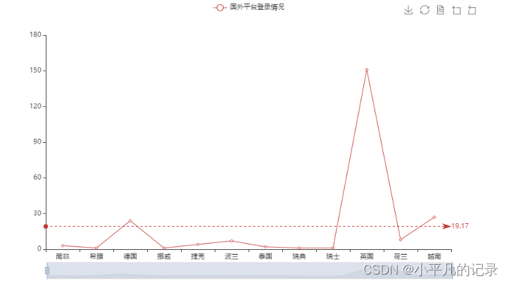
——国外
#各国登录统计
Login_he2 =  Login_he.groupby(by='guobie',as_index=False).count()
#不包括中国
Login_he3 = Login_he2[~Login_he2['guobie'].isin(["中国"])]
Login_he3
.dataframe tbody tr th {
    vertical-align: top;
}

.dataframe thead th {
    text-align: right;
}
| guobie | user_id | login_time | shengfen | chengshi | |
|---|---|---|---|---|---|
| 1 | 南非 | 3 | 3 | 3 | 3 |
| 2 | 希腊 | 1 | 1 | 1 | 1 |
| 3 | 德国 | 24 | 24 | 24 | 24 |
| 4 | 挪威 | 1 | 1 | 1 | 1 |
| 5 | 捷克 | 4 | 4 | 4 | 4 |
| 6 | 波兰 | 7 | 7 | 7 | 7 |
| 7 | 泰国 | 2 | 2 | 2 | 2 |
| 8 | 瑞典 | 1 | 1 | 1 | 1 |
| 9 | 瑞士 | 1 | 1 | 1 | 1 |
| 10 | 英国 | 151 | 151 | 151 | 151 |
| 11 | 荷兰 | 8 | 8 | 8 | 8 |
| 12 | 越南 | 27 | 27 | 27 | 27 |
from pyecharts.charts import Line
from pyecharts import options as opts
x_data = list(Login_he3['guobie'])
#['South Africa','Greece','Germany','Norway','Czech Rep.','Poland','Thailand',
         # 'Sweden','Switzerland','United Kingdom','Netherlands','Vietnam']
y_data = Login_he3['user_id']

# 特殊值标记
line = (Line()
        .add_xaxis(x_data)
        .add_yaxis("国外平台登录情况",y_data)
        .set_series_opts(
        # 为了不影响标记点,这里把标签关掉
        label_opts=opts.LabelOpts(is_show=False),
        markline_opts=opts.MarkLineOpts(
            data=[
                opts.MarkLineItem(type_="average", name="平均值")
            ]))
        .set_global_opts(
            #title_opts=opts.TitleOpts(title="国内平台登录次数", subtitle="副标题"),                         # 标题
            toolbox_opts=opts.ToolboxOpts(),                                 # 工具箱
            datazoom_opts=opts.DataZoomOpts(range_start=0,range_end=100)     # 横轴缩放
        )
        )
line.render_notebook()
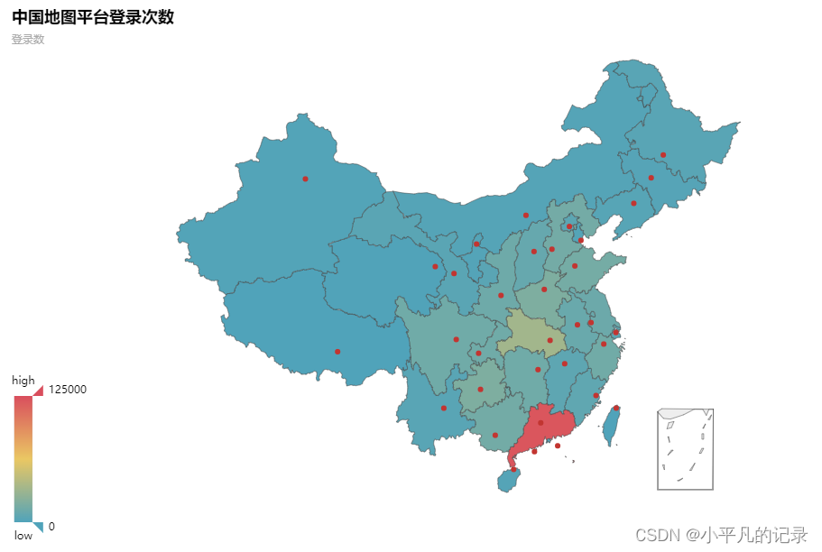
各省份平台登录次数热力地图
#不包括国外
Login_china = Login_he[Login_he['guobie'].isin(["中国"])]

Login_china2 =  Login_china.groupby(by='shengfen',as_index=False).count()
Login_china3 = Login_china2.iloc[1:,]
Login_china3['count'] = Login_china3['user_id']
Login_china3.head()
.dataframe tbody tr th {
    vertical-align: top;
}

.dataframe thead th {
    text-align: right;
}
| shengfen | user_id | login_time | guobie | chengshi | count | |
|---|---|---|---|---|---|---|
| 1 | 上海 | 5365 | 5365 | 5365 | 5365 | 5365 |
| 2 | 云南 | 3750 | 3750 | 3750 | 3750 | 3750 |
| 3 | 内蒙 | 1870 | 1870 | 1870 | 1870 | 1870 |
| 4 | 内蒙古 | 1870 | 1870 | 1870 | 1870 | 1870 |
| 5 | 北京 | 4946 | 4946 | 4946 | 4946 | 4946 |
type(y_data.values)
numpy.ndarray
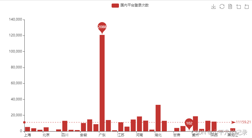
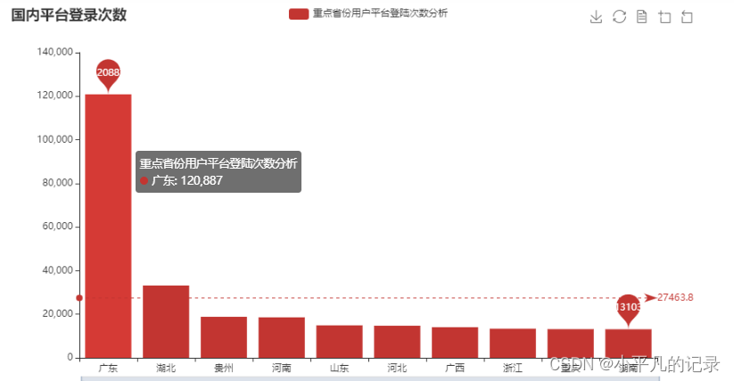
——全国省份用户登录人数分布
from pyecharts.charts import Bar

x_data = list(Login_china3['shengfen'])
y_data = list(Login_china3['count'])

# 特殊值标记
bar = (Bar()
       .add_xaxis(x_data)
       .add_yaxis('国内平台登录次数', y_data)
       .set_series_opts(
        markpoint_opts=opts.MarkPointOpts(
            data=[
                opts.MarkPointItem(type_="max", name="最大值"),
                opts.MarkPointItem(type_="min", name="最小值"),
            ]))
       .set_global_opts(
            #title_opts=opts.TitleOpts(title="国内平台登录次数", subtitle="副标题"),                         # 标题
            toolbox_opts=opts.ToolboxOpts(),                 # 工具箱
            datazoom_opts=opts.DataZoomOpts(range_start=0,range_end=100)     # 横轴缩放
        )
       .set_series_opts(
        # 为了不影响标记点,这里把标签关掉
        label_opts=opts.LabelOpts(is_show=False),
        markline_opts=opts.MarkLineOpts(
            data=[
                opts.MarkLineItem(type_="average", name="平均值")
            ]))
      )

bar.render_notebook()
#bar.render('map2.html') #保存到本地
from pyecharts.charts import Map
province = ['北京市','天津市','河北省','山西省','内蒙古自治区','辽宁省','吉林省','黑龙江省','上海市','江苏省','浙江省','安徽省','福建省','江西省',
'山东省','河南省','湖北省','湖南省','广东省','广西壮族自治区','海南省','重庆市','四川省','贵州省','云南省','陕西省','甘肃省','青海省','宁夏回族自治区','新疆维吾尔自治区']

values = list(Login_china3['count'])
data = [[province[i],values[i]] for i in range(len(province))]
map = (
    Map()
    .add("中国地图平台登录次数",data,'china')
      )
map.set_global_opts(
    visualmap_opts=opts.VisualMapOpts(max_=125000),  #最大数据范围
    toolbox_opts=opts.ToolboxOpts()                                                     # 工具箱
    )
map.render_notebook()
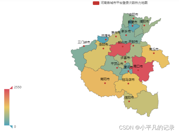
各城市平台登录次数热力地图
#重点省份用户平台登陆次数分析

Login_china4 = Login_china3.sort_values(by='count',ascending=False)
Login_china5 = Login_china4.iloc[0:10,:]

x_data = list(Login_china5['shengfen'])
y_data = list(Login_china5['count'])

bar = (Bar()
       .add_xaxis(x_data)
       .add_yaxis('重点省份用户平台登陆次数分析', y_data)
       .set_series_opts(
        markpoint_opts=opts.MarkPointOpts(
            data=[
                opts.MarkPointItem(type_="max", name="最大值"),
                opts.MarkPointItem(type_="min", name="最小值"),
            ]))
       .set_global_opts(
            title_opts=opts.TitleOpts(title="国内平台登录次数"),                         # 标题
            toolbox_opts=opts.ToolboxOpts(),                                                     # 工具箱
            datazoom_opts=opts.DataZoomOpts(range_start=0,range_end=100)                         # 横轴缩放
        )
       .set_series_opts(
        # 为了不影响标记点,这里把标签关掉
        label_opts=opts.LabelOpts(is_show=False),
        markline_opts=opts.MarkLineOpts(
            data=[
                opts.MarkLineItem(type_="average", name="平均值")
            ]))
      )
bar.render_notebook()
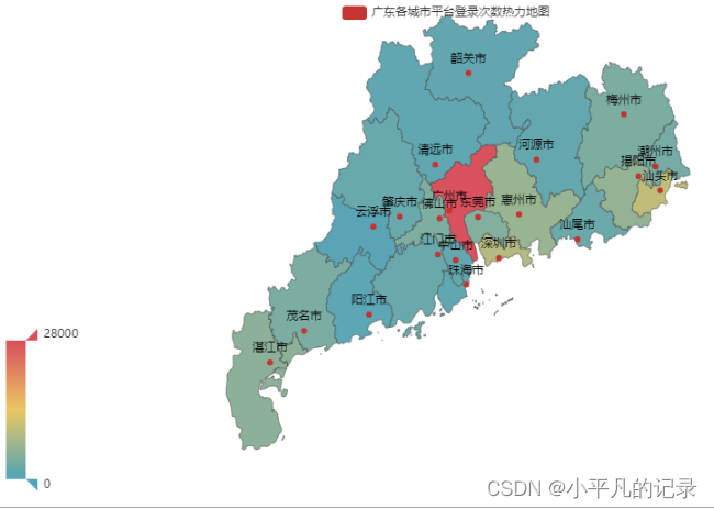
——重点省份用户分布情况分析
#广东
Login_guangdong1 = Login_he[Login_he['shengfen'].isin(["广东"])]
Login_guangdong2 =  Login_guangdong1.groupby(by='chengshi',as_index=False).count()
Login_guangdong = Login_guangdong2.iloc[1:,]

Login_guangdong["new_chengshi"] = Login_guangdong['chengshi']+'市'

x_data = list(Login_guangdong['user_id'])
y_data = list(Login_guangdong['new_chengshi'])
data = [[y_data[i],x_data[i]] for i in range(len(y_data))]

map = (
    Map()
    .add("广东各城市平台登录次数热力地图",data,'广东')
      )
map.set_global_opts(
    visualmap_opts=opts.VisualMapOpts(max_=28000),  #最大数据范围
    toolbox_opts=opts.ToolboxOpts()                                                     # 工具箱
    )
map.render_notebook()
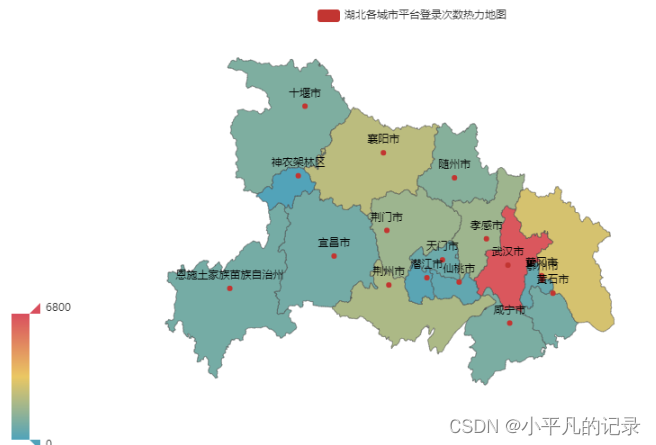
#湖北

Login_hubei1 = Login_he[Login_he['shengfen'].isin(["湖北"])]
Login_hubei2 =  Login_hubei1.groupby(by='chengshi',as_index=False).count()
Login_hubei = Login_hubei2.iloc[1:,]

Login_hubei["new_chengshi"] = Login_hubei['chengshi']+'市'
Login_hubei.loc[Login_hubei['new_chengshi']== '恩施土家族苗族自治州市','new_chengshi']= '恩施土家族苗族自治州'
Login_hubei.loc[Login_hubei['new_chengshi']== '神农架林区市','new_chengshi']= '神农架林区'
x_data = list(Login_hubei['user_id'])
y_data = list(Login_hubei['new_chengshi'])

data = [[y_data[i],x_data[i]] for i in range(len(y_data))]

map = (
    Map()
    .add("湖北各城市平台登录次数热力地图",data,'湖北')
      )
map.set_global_opts(
    visualmap_opts=opts.VisualMapOpts(max_=6800),  #最大数据范围
    toolbox_opts=opts.ToolboxOpts()                                                     # 工具箱
    )
map.render_notebook()
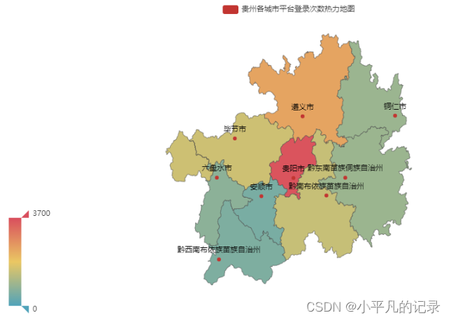
#贵州

Login_guizhou1 = Login_he[Login_he['shengfen'].isin(["贵州"])]
Login_guizhou2 =  Login_guizhou1.groupby(by='chengshi',as_index=False).count()
Login_guizhou = Login_guizhou2.iloc[1:,]

Login_guizhou["new_chengshi"] = Login_guizhou['chengshi']+'市'
Login_guizhou.loc[Login_guizhou['new_chengshi']== '黔东南苗族侗族自治州市','new_chengshi']= '黔东南苗族侗族自治州'
Login_guizhou.loc[Login_guizhou['new_chengshi']== '黔南布依族苗族自治州市','new_chengshi']= '黔南布依族苗族自治州'
Login_guizhou.loc[Login_guizhou['new_chengshi']== '黔西南布依族苗族自治州市','new_chengshi']= '黔西南布依族苗族自治州'

x_data = list(Login_guizhou['user_id'])
y_data = list(Login_guizhou['new_chengshi'])

data = [[y_data[i],x_data[i]] for i in range(len(y_data))]

map = (
    Map()
    .add("贵州各城市平台登录次数热力地图",data,'贵州')
      )
map.set_global_opts(
    visualmap_opts=opts.VisualMapOpts(max_=3700),  #最大数据范围
    toolbox_opts=opts.ToolboxOpts()                                                     # 工具箱
    )
map.render_notebook()
#河南

Login_henan1 = Login_he[Login_he['shengfen'].isin(["河南"])]
Login_henan2 =  Login_henan1.groupby(by='chengshi',as_index=False).count()
Login_henan = Login_henan2.iloc[1:,]

Login_henan["new_chengshi"] = Login_henan['chengshi']+'市'

x_data = list(Login_henan['user_id'])
y_data = list(Login_henan['new_chengshi'])

data = [[y_data[i],x_data[i]] for i in range(len(y_data))]

map = (
    Map()
    .add("河南各城市平台登录次数热力地图",data,'河南')
      )
map.set_global_opts(
    visualmap_opts=opts.VisualMapOpts(max_=2550),  #最大数据范围
    toolbox_opts=opts.ToolboxOpts()                                                     # 工具箱
    )
map.render_notebook()
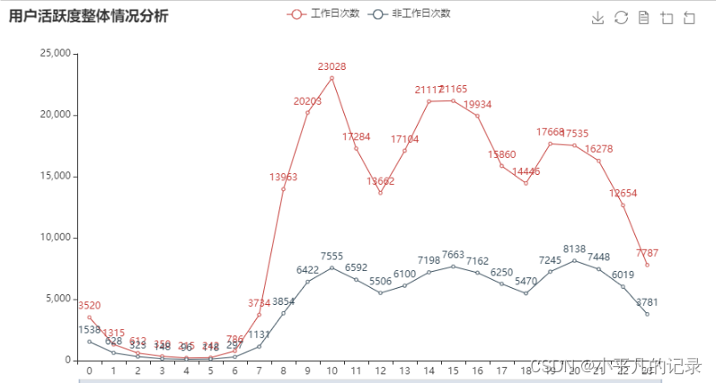
任务 2.2
分别绘制工作日与非工作日各时段的用户登录次数柱状图,并分析用户活跃的主要时间段。
#将日期与时间分割
Login1 = Login["login_time"].str.split(" ",expand=True).fillna("")
Login1['login_data'] = Login1[0]
Login1['login_hour'] = Login1[1]
Login1['user_id'] = Login['user_id']
Login2 = Login1[['user_id','login_data','login_hour']]
Login2.head()
.dataframe tbody tr th {
    vertical-align: top;
}

.dataframe thead th {
    text-align: right;
}
| user_id | login_data | login_hour | |
|---|---|---|---|
| 0 | 用户3 | 2018-09-06 | 09:32:47 |
| 1 | 用户3 | 2018-09-07 | 09:28:28 |
| 2 | 用户3 | 2018-09-07 | 09:57:44 |
| 3 | 用户3 | 2018-09-07 | 10:55:07 |
| 4 | 用户3 | 2018-09-07 | 12:28:42 |
工作日分析
import datetime
import chinese_calendar

start_time = datetime.datetime(2018, 9, 6)
end_time = datetime.datetime(2020, 6, 18)

#获取工作日时期
a = chinese_calendar.get_workdays(start_time,end_time)
#chinese_calendar.get_holidays(start_time,end_time)

#转换为日期列表
date_string = [d.strftime('%Y-%m-%d') for d in a]

#筛选工作日所含数据
Login3 = Login2[Login2['login_data'].isin(date_string)]

#将小时取整
x = Login3['login_hour']
Login3['login_newhour'] = Login3['login_hour'].apply(lambda x: int(x[0:2]))
Login3.head()
.dataframe tbody tr th {
    vertical-align: top;
}

.dataframe thead th {
    text-align: right;
}
| user_id | login_data | login_hour | login_newhour | |
|---|---|---|---|---|
| 0 | 用户3 | 2018-09-06 | 09:32:47 | 9 |
| 1 | 用户3 | 2018-09-07 | 09:28:28 | 9 |
| 2 | 用户3 | 2018-09-07 | 09:57:44 | 9 |
| 3 | 用户3 | 2018-09-07 | 10:55:07 | 10 |
| 4 | 用户3 | 2018-09-07 | 12:28:42 | 12 |
gongzuori = Login3.groupby(by=Login3['login_newhour'],as_index=False)['user_id'].count()
gongzuori['gongzuori'] = gongzuori['user_id']
gongzuori = gongzuori[['login_newhour','gongzuori']]
gongzuori.head()
.dataframe tbody tr th {
    vertical-align: top;
}

.dataframe thead th {
    text-align: right;
}
| login_newhour | gongzuori | |
|---|---|---|
| 0 | 0 | 3520 |
| 1 | 1 | 1315 |
| 2 | 2 | 612 |
| 3 | 3 | 350 |
| 4 | 4 | 215 |
非工作日分析
import datetime
import chinese_calendar

start_time = datetime.datetime(2018, 9, 6)
end_time = datetime.datetime(2020, 6, 18)

#获取工作日时期
a = chinese_calendar.get_holidays(start_time,end_time)
#chinese_calendar.get_holidays(start_time,end_time)

#转换为日期列表
date_string = [d.strftime('%Y-%m-%d') for d in a]

#筛选工作日所含数据
Login4 = Login2[Login2['login_data'].isin(date_string)]

#将小时取整
x = Login4['login_hour']
Login4['login_newhour'] = Login4['login_hour'].apply(lambda x: int(x[0:2]))
Login4.head()
.dataframe tbody tr th {
    vertical-align: top;
}

.dataframe thead th {
    text-align: right;
}
| user_id | login_data | login_hour | login_newhour | |
|---|---|---|---|---|
| 38 | 用户3 | 2018-09-23 | 00:56:32 | 0 |
| 88 | 用户3 | 2018-10-13 | 09:19:45 | 9 |
| 89 | 用户3 | 2018-10-13 | 16:02:59 | 16 |
| 104 | 用户3 | 2018-10-20 | 17:10:33 | 17 |
| 135 | 用户3 | 2018-11-04 | 18:02:06 | 18 |
holidays = Login4.groupby(by=Login4['login_newhour'],as_index=False)['user_id'].count()
holidays['holidays'] = holidays['user_id']
holidays = holidays[['login_newhour','holidays']]
holidays.head()
.dataframe tbody tr th {
    vertical-align: top;
}

.dataframe thead th {
    text-align: right;
}
| login_newhour | holidays | |
|---|---|---|
| 0 | 0 | 1538 |
| 1 | 1 | 628 |
| 2 | 2 | 323 |
| 3 | 3 | 148 |
| 4 | 4 | 96 |
from pyecharts.charts import Line
attr = list(gongzuori['login_newhour'])
v1 = list(gongzuori['gongzuori'])
v2 = list(holidays['holidays'])

line = (Line()
       .add_xaxis(attr)
       .add_yaxis('工作日次数', v1)
       .add_yaxis('非工作日次数',v2)
       .set_global_opts(
            title_opts=opts.TitleOpts(title="用户活跃度整体情况分析"),       # 标题
            toolbox_opts=opts.ToolboxOpts(),                               # 工具箱
            datazoom_opts=opts.DataZoomOpts(range_start=0,range_end=100)    # 横轴缩放
        )
      )
line.render_notebook()
任务 2.3
记𝑇end为数据观察窗口截止时间(如:赛题数据的采集截止时间为2020 年 6 月 18 日),𝑇𝑖为用户 i 的最近访问时间,𝜎𝑖 = 𝑇end − 𝑇𝑖,若𝜎𝑖 > 90天,则称用户 i 为流失用户。根据该定义计算平台用户的流失率。
用户总体情况分析
Tend = pd.date_range('20200618235959',periods=1)
new_users.drop_duplicates(inplace=True)
new_users['Tend'] = list(Tend)*43909
new_users['longtime'] = (pd.to_datetime(new_users['Tend']) - pd.to_datetime(new_users['recently_logged'])).map(lambda x:x.days)
#new_users['longtime'] = new_users['longtime'].astype(str)
new_users3 = new_users.dropna()
#new_users['longtime'].str.split("",expand=True).fillna("")
new_users3.head()
.dataframe tbody tr th {
    vertical-align: top;
}

.dataframe thead th {
    text-align: right;
}
| user_id | register_time | recently_logged | number_of_classes_join | number_of_classes_out | learn_time | Tend | longtime | |
|---|---|---|---|---|---|---|---|---|
| 0 | 用户44251 | 2020/6/18 9:49 | 2020/6/18 9:49 | 0 | 0 | 41.25 | 2020-06-18 23:59:59 | 0.0 |
| 1 | 用户44250 | 2020/6/18 9:47 | 2020/6/18 9:48 | 0 | 0 | 0 | 2020-06-18 23:59:59 | 0.0 |
| 2 | 用户44249 | 2020/6/18 9:43 | 2020/6/18 9:43 | 0 | 0 | 16.22 | 2020-06-18 23:59:59 | 0.0 |
| 3 | 用户44248 | 2020/6/18 9:09 | 2020/6/18 9:09 | 0 | 0 | 0 | 2020-06-18 23:59:59 | 0.0 |
| 4 | 用户44247 | 2020/6/18 7:41 | 2020/6/18 8:15 | 0 | 0 | 1.8 | 2020-06-18 23:59:59 | 0.0 |
new_users3['longtime'].describe()
count    43717.000000
mean       190.146259
std        170.868948
min          0.000000
25%         49.000000
50%        115.000000
75%        343.000000
max        646.000000
Name: longtime, dtype: float64
new_users4 =  new_users3.groupby(by='longtime',as_index=False).count()

x_data = list(new_users4['longtime'])
y_data = list(new_users4['user_id'])

bar = (Bar()
       .add_xaxis(x_data)
       .add_yaxis('人数', y_data)
       .set_series_opts(
        # 为了不影响标记点,这里把标签关掉
        label_opts=opts.LabelOpts(is_show=False))
       .set_global_opts(
            title_opts=opts.TitleOpts(title="各类时间差值人数分析"),      # 标题
            toolbox_opts=opts.ToolboxOpts(),                             # 工具箱
            datazoom_opts=opts.DataZoomOpts(range_start=0,range_end=100) # 横轴缩放
        )
      )
bar.render_notebook()
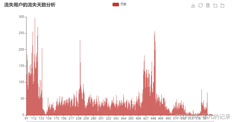
流失天数及流失率分析
new_users5  = new_users3[new_users3['longtime'] >90]

new_users6 =  new_users5.groupby(by='longtime',as_index=False).count()

x_data = list(new_users6['longtime'])
y_data = list(new_users6['user_id'])

bar = (Bar()
       .add_xaxis(x_data)
       .add_yaxis('天数', y_data)
       .set_series_opts(
        # 为了不影响标记点,这里把标签关掉
        label_opts=opts.LabelOpts(is_show=False))
       .set_global_opts(
            title_opts=opts.TitleOpts(title="流失用户的流失天数分析"),                         # 标题
            toolbox_opts=opts.ToolboxOpts(),                                                     # 工具箱
            datazoom_opts=opts.DataZoomOpts(range_start=0,range_end=100)                         # 横轴缩放
        )
      )
bar.render_notebook()

print('流失率:',new_users5['longtime'].count()/43717)
print('流失人数:',new_users5['longtime'].count())
流失率: 0.5796143376718439
流失人数: 25339
未流失客户流失风险等级分类分析
潜水用户:小于 90 天且大于 60 天
活跃用户:小于 60 天
高活跃用户:小于 30 天

低活跃用户:小于 60 天且大于 30 天
qianshui = new_users3[(new_users3.longtime > 60) & (new_users3.longtime < 90)]['longtime'].count()
print('潜水用户:',qianshui)
print('潜水用户占比:',qianshui/(43717-25339))
潜水用户: 4796
潜水用户占比: 0.260964196321689
gao_huoyue = new_users3[new_users3.longtime < 30]['longtime'].count()
print('高活跃用户:',gao_huoyue)
print('高活跃用户占比:',gao_huoyue/(43717-25339))
高活跃用户: 7516
高活跃用户占比: 0.40896724344324736
di_huoyue = new_users3[(new_users3.longtime > 30) & (new_users3.longtime < 60)]['longtime'].count()
print('低活跃用户:',di_huoyue)
print('低活跃用户占比:',di_huoyue/(43717-25339))
低活跃用户: 5647
低活跃用户占比: 0.3072695614321471
任务 2.4
根据任务 2.1 至任务 2.3,分析平台用户的活跃度,为该教育平台
的线上管理决策提供建议。
任务 3 线上课程推荐
任务 3.1
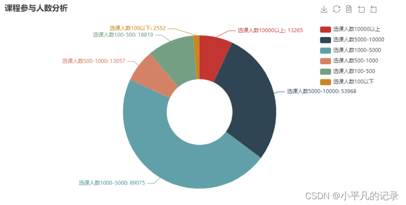
根据用户参与学习的记录,统计每门课程的参与人数,计算每门课程的受欢迎程度,列出最受欢迎的前 10 门课程,并绘制相应的柱图。
study_information1= study_information.groupby(by='course_id',as_index=False)['user_id'].count()
study_information1['num'] = study_information1['user_id']
study_information2 = study_information1[['course_id','num']]
study_information2.head()
.dataframe tbody tr th {
    vertical-align: top;
}

.dataframe thead th {
    text-align: right;
}
| course_id | num | |
|---|---|---|
| 0 | 课程0 | 2 |
| 1 | 课程1 | 4 |
| 2 | 课程10 | 35 |
| 3 | 课程100 | 5 |
| 4 | 课程101 | 482 |
选课人数分析
study_information2['num'].sum()
190736
num1 = study_information2[(study_information2.num > 10000)]['num'].sum()
print('选课人数10000以上:',num1)
print('选课人数占比:',num1/190736)
选课人数10000以上: 13265
选课人数占比: 0.06954638872577804
num2 = study_information2[(study_information2.num > 5000) & (study_information2.num < 10000)]['num'].sum()
print('选课人数5000-10000:',num2)
print('选课人数占比:',num2/190736)
选课人数5000-10000: 53968
选课人数占比: 0.2829460615720158
num3 = study_information2[(study_information2.num > 1000) & (study_information2.num < 5000)]['num'].sum()
print('选课人数1000-5000:',num3)
print('选课人数占比:',num3/190736)
选课人数1000-5000: 89075
选课人数占比: 0.4670067527891955
num4 = study_information2[(study_information2.num > 500) & (study_information2.num < 1000)]['num'].sum()
print('选课人数500-1000:',num4)
print('选课人数占比:',num4/190736)
选课人数500-1000: 13057
选课人数占比: 0.06845587618488382
num5 = study_information2[(study_information2.num > 100) & (study_information2.num < 500)]['num'].sum()
print('选课人数100-500:',num5)
print('选课人数占比:',num5/190736)
选课人数100-500: 18819
选课人数占比: 0.09866517070715544
num6 = study_information2[(study_information2.num < 100)]['num'].sum()
print('选课人数100以下:',num6)
print('选课人数占比:',num6/190736)
选课人数100以下: 2552
选课人数占比: 0.013379750020971396
from pyecharts.charts import Pie
x_data = ["选课人数10000以上", "选课人数5000-10000", "选课人数1000-5000", "选课人数500-1000", "选课人数100-500","选课人数100以下"]
y_data = [13265, 53968, 89075, 13057, 18819,2552]

c = (
    Pie()
    .add("", [list(z) for z in zip(x_data, y_data)],radius=["30%", "70%"])   # zip函数两个部分组合在一起list(zip(x,y))-----> [(x,y)]
    .set_global_opts(
        title_opts=opts.TitleOpts(title="课程参与人数分析"), # 标题
        toolbox_opts=opts.ToolboxOpts(),                                                     # 工具箱
        legend_opts=opts.LegendOpts(orient="vertical", pos_top="10%", pos_left="80%")) #图例设置
    .set_series_opts(label_opts=opts.LabelOpts(formatter="{b}: {c}"))  # 数据标签设置
    )
c.render_notebook()
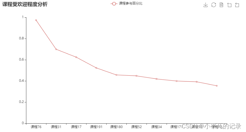
课程受欢迎程度分析
study_information2.describe()
.dataframe tbody tr th {
    vertical-align: top;
}

.dataframe thead th {
    text-align: right;
}
| num | |
|---|---|
| count | 239.000000 |
| mean | 798.058577 |
| std | 1746.098741 |
| min | 1.000000 |
| 25% | 18.500000 |
| 50% | 138.000000 |
| 75% | 458.500000 |
| max | 13265.000000 |
study_information2['y'] = (study_information2['num']-1)/13624
study_information2 = study_information2.sort_values(by='y',ascending=False)
study_information3 = study_information2.iloc[0:10,:]
study_information3
.dataframe tbody tr th {
    vertical-align: top;
}

.dataframe thead th {
    text-align: right;
}
| course_id | num | y | |
|---|---|---|---|
| 214 | 课程76 | 13265 | 0.973576 |
| 166 | 课程31 | 9521 | 0.698767 |
| 79 | 课程17 | 8505 | 0.624193 |
| 103 | 课程191 | 7126 | 0.522974 |
| 91 | 课程180 | 6223 | 0.456694 |
| 188 | 课程52 | 6105 | 0.448033 |
| 169 | 课程34 | 5709 | 0.418967 |
| 81 | 课程171 | 5437 | 0.399002 |
| 187 | 课程50 | 5342 | 0.392029 |
| 24 | 课程12 | 4829 | 0.354375 |
x_data = list(study_information3['course_id'])
y_data_line = list(study_information3['y'])

line = (Line()
       .add_xaxis(x_data)
       .add_yaxis('课程参与百分比', y_data_line)
       .set_global_opts(
            title_opts=opts.TitleOpts(title="课程受欢迎程度分析"),                         # 标题
            toolbox_opts=opts.ToolboxOpts()                                                     # 工具箱
        )
       .set_series_opts(
        # 为了不影响标记点,这里把标签关掉
        label_opts=opts.LabelOpts(is_show=False))
      )
line.render_notebook()
x_data = list(study_information3['course_id'])
y_data_line = list(round(study_information3['y'],2))


c = (
    Pie()
    .add("", [list(z) for z in zip(x_data, y_data_line)],
         center=['45%', '55%'],radius=["25%", "70%"],rosetype="area")   # zip函数两个部分组合在一起list(zip(x,y))-----> [(x,y)]
    .set_global_opts(
        title_opts=opts.TitleOpts(title="课程受欢迎程度分析"), # 标题
        toolbox_opts=opts.ToolboxOpts(),                                                     # 工具箱
        legend_opts=opts.LegendOpts(orient="vertical", pos_top="10%", pos_left="80%")) #图例设置
    .set_series_opts(label_opts=opts.LabelOpts(formatter="{b}:{c}"))  # 数据标签设置
    )
c.render_notebook()
任务 3.2
根据用户选择课程情况,构建用户和课程的关系表(二元矩阵),使用基于物品的协同过滤算法计算课程之间的相似度,并结合用户已选课程的记录,为总学习进度最高的 5 名用户推荐 3 门课程。
构建用户和课程的关系表(二元矩阵)
study_information['num'] =1

study_information4 = study_information[['user_id','course_id','num']]
study_information5 = study_information4.pivot(index='user_id',columns='course_id',values='num').fillna(0)
study_information5
.dataframe tbody tr th {
    vertical-align: top;
}

.dataframe thead th {
    text-align: right;
}
| course_id | 课程0 | 课程1 | 课程10 | 课程100 | 课程101 | 课程102 | 课程103 | 课程104 | 课程105 | 课程106 | ... | 课程9 | 课程90 | 课程91 | 课程92 | 课程93 | 课程94 | 课程95 | 课程97 | 课程98 | 课程99 |
|---|---|---|---|---|---|---|---|---|---|---|---|---|---|---|---|---|---|---|---|---|---|
| user_id | |||||||||||||||||||||
| 用户10 | 0.0 | 0.0 | 0.0 | 0.0 | 0.0 | 0.0 | 0.0 | 0.0 | 0.0 | 0.0 | ... | 0.0 | 0.0 | 0.0 | 0.0 | 0.0 | 0.0 | 0.0 | 0.0 | 0.0 | 0.0 |
| 用户100 | 0.0 | 0.0 | 0.0 | 0.0 | 0.0 | 0.0 | 0.0 | 0.0 | 0.0 | 0.0 | ... | 0.0 | 0.0 | 0.0 | 0.0 | 0.0 | 0.0 | 0.0 | 0.0 | 0.0 | 0.0 |
| 用户10000 | 0.0 | 0.0 | 0.0 | 0.0 | 0.0 | 0.0 | 0.0 | 0.0 | 0.0 | 0.0 | ... | 0.0 | 0.0 | 0.0 | 0.0 | 0.0 | 0.0 | 0.0 | 0.0 | 0.0 | 0.0 |
| 用户10001 | 0.0 | 0.0 | 0.0 | 0.0 | 0.0 | 0.0 | 0.0 | 0.0 | 0.0 | 0.0 | ... | 0.0 | 0.0 | 0.0 | 0.0 | 0.0 | 0.0 | 0.0 | 0.0 | 0.0 | 0.0 |
| 用户10002 | 0.0 | 0.0 | 0.0 | 0.0 | 0.0 | 0.0 | 0.0 | 0.0 | 0.0 | 0.0 | ... | 0.0 | 0.0 | 0.0 | 0.0 | 0.0 | 0.0 | 0.0 | 0.0 | 0.0 | 0.0 |
| ... | ... | ... | ... | ... | ... | ... | ... | ... | ... | ... | ... | ... | ... | ... | ... | ... | ... | ... | ... | ... | ... |
| 用户9993 | 0.0 | 0.0 | 0.0 | 0.0 | 0.0 | 0.0 | 0.0 | 0.0 | 0.0 | 0.0 | ... | 0.0 | 0.0 | 0.0 | 0.0 | 0.0 | 0.0 | 0.0 | 0.0 | 0.0 | 0.0 |
| 用户9994 | 0.0 | 0.0 | 0.0 | 0.0 | 0.0 | 0.0 | 0.0 | 0.0 | 0.0 | 0.0 | ... | 0.0 | 0.0 | 0.0 | 0.0 | 0.0 | 0.0 | 0.0 | 0.0 | 0.0 | 0.0 |
| 用户9995 | 0.0 | 0.0 | 0.0 | 0.0 | 0.0 | 0.0 | 0.0 | 0.0 | 0.0 | 0.0 | ... | 0.0 | 0.0 | 0.0 | 0.0 | 0.0 | 0.0 | 0.0 | 0.0 | 0.0 | 0.0 |
| 用户9996 | 0.0 | 0.0 | 0.0 | 0.0 | 1.0 | 0.0 | 0.0 | 0.0 | 0.0 | 0.0 | ... | 0.0 | 0.0 | 0.0 | 0.0 | 0.0 | 0.0 | 0.0 | 0.0 | 0.0 | 0.0 |
| 用户9999 | 0.0 | 0.0 | 0.0 | 0.0 | 0.0 | 0.0 | 0.0 | 0.0 | 0.0 | 0.0 | ... | 0.0 | 0.0 | 0.0 | 0.0 | 0.0 | 0.0 | 0.0 | 0.0 | 0.0 | 0.0 |
40373 rows × 239 columns
物品的协同过滤算法
from sklearn.metrics import jaccard_score

items = study_information5.columns
from sklearn.metrics.pairwise import pairwise_distances
# 计算课程间相似度
course_similar = 1 - pairwise_distances(study_information5.T.values,metric="jaccard")
course_similar = pd.DataFrame(course_similar, columns=items, index=items)

course_similar
.dataframe tbody tr th {
    vertical-align: top;
}

.dataframe thead th {
    text-align: right;
}
| course_id | 课程0 | 课程1 | 课程10 | 课程100 | 课程101 | 课程102 | 课程103 | 课程104 | 课程105 | 课程106 | ... | 课程9 | 课程90 | 课程91 | 课程92 | 课程93 | 课程94 | 课程95 | 课程97 | 课程98 | 课程99 |
|---|---|---|---|---|---|---|---|---|---|---|---|---|---|---|---|---|---|---|---|---|---|
| course_id | |||||||||||||||||||||
| 课程0 | 1.000000 | 0.500000 | 0.027778 | 0.400000 | 0.000000 | 0.666667 | 1.000000 | 1.000000 | 0.250000 | 0.000000 | ... | 1.000000 | 0.000000 | 0.000000 | 0.000000 | 0.000000 | 0.001934 | 0.008621 | 0.005556 | 0.003484 | 0.005291 |
| 课程1 | 0.500000 | 1.000000 | 0.026316 | 0.285714 | 0.002062 | 0.400000 | 0.500000 | 0.500000 | 0.166667 | 0.000000 | ... | 0.500000 | 0.000000 | 0.000000 | 0.000000 | 0.000000 | 0.001931 | 0.008475 | 0.011050 | 0.005217 | 0.010526 |
| 课程10 | 0.027778 | 0.026316 | 1.000000 | 0.052632 | 0.001938 | 0.027027 | 0.027778 | 0.027778 | 0.027027 | 0.002475 | ... | 0.027778 | 0.000000 | 0.000000 | 0.028571 | 0.000000 | 0.031853 | 0.171875 | 0.086294 | 0.032203 | 0.087805 |
| 课程100 | 0.400000 | 0.285714 | 0.052632 | 1.000000 | 0.002058 | 0.600000 | 0.400000 | 0.400000 | 0.142857 | 0.000000 | ... | 0.400000 | 0.000000 | 0.000000 | 0.000000 | 0.000000 | 0.003865 | 0.016949 | 0.010989 | 0.006957 | 0.015789 |
| 课程101 | 0.000000 | 0.002062 | 0.001938 | 0.002058 | 1.000000 | 0.000000 | 0.000000 | 0.000000 | 0.000000 | 0.000000 | ... | 0.000000 | 0.000000 | 0.000000 | 0.002075 | 0.000000 | 0.014047 | 0.003361 | 0.021638 | 0.067745 | 0.021341 |
| ... | ... | ... | ... | ... | ... | ... | ... | ... | ... | ... | ... | ... | ... | ... | ... | ... | ... | ... | ... | ... | ... |
| 课程94 | 0.001934 | 0.001931 | 0.031853 | 0.003865 | 0.014047 | 0.001932 | 0.001934 | 0.001934 | 0.000965 | 0.120511 | ... | 0.001934 | 0.000967 | 0.000000 | 0.000967 | 0.000967 | 1.000000 | 0.092205 | 0.034983 | 0.145299 | 0.037351 |
| 课程95 | 0.008621 | 0.008475 | 0.171875 | 0.016949 | 0.003361 | 0.008547 | 0.008621 | 0.008621 | 0.008547 | 0.000000 | ... | 0.008621 | 0.008696 | 0.000000 | 0.000000 | 0.000000 | 0.092205 | 1.000000 | 0.076923 | 0.063272 | 0.082143 |
| 课程97 | 0.005556 | 0.011050 | 0.086294 | 0.010989 | 0.021638 | 0.005525 | 0.005556 | 0.005556 | 0.005525 | 0.001825 | ... | 0.005556 | 0.005587 | 0.000000 | 0.005587 | 0.000000 | 0.034983 | 0.076923 | 1.000000 | 0.261307 | 0.882051 |
| 课程98 | 0.003484 | 0.005217 | 0.032203 | 0.006957 | 0.067745 | 0.003478 | 0.003484 | 0.003484 | 0.001736 | 0.040794 | ... | 0.003484 | 0.001742 | 0.001742 | 0.000000 | 0.001742 | 0.145299 | 0.063272 | 0.261307 | 1.000000 | 0.261589 |
| 课程99 | 0.005291 | 0.010526 | 0.087805 | 0.015789 | 0.021341 | 0.010582 | 0.005291 | 0.005291 | 0.005263 | 0.001795 | ... | 0.005291 | 0.005319 | 0.000000 | 0.005319 | 0.000000 | 0.037351 | 0.082143 | 0.882051 | 0.261589 | 1.000000 |
239 rows × 239 columns
topN_items = {}
# 遍历每一行数据
for i in course_similar.index:
    # 取出每一列数据,并删除自身,然后排序数据
    _df = course_similar.loc[i].drop([i])
    _df_sorted = _df.sort_values(ascending=False)

    top2 = list(_df_sorted.index[:3])
    topN_items[i] = top2

topN_items = pd.DataFrame(topN_items,columns=items)
topN_items
.dataframe tbody tr th {
    vertical-align: top;
}

.dataframe thead th {
    text-align: right;
}
| course_id | 课程0 | 课程1 | 课程10 | 课程100 | 课程101 | 课程102 | 课程103 | 课程104 | 课程105 | 课程106 | ... | 课程9 | 课程90 | 课程91 | 课程92 | 课程93 | 课程94 | 课程95 | 课程97 | 课程98 | 课程99 |
|---|---|---|---|---|---|---|---|---|---|---|---|---|---|---|---|---|---|---|---|---|---|
| 0 | 课程41 | 课程142 | 课程140 | 课程102 | 课程71 | 课程84 | 课程0 | 课程0 | 课程0 | 课程109 | ... | 课程0 | 课程205 | 课程45 | 课程30 | 课程234 | 课程117 | 课程38 | 课程99 | 课程7 | 课程97 |
| 1 | 课程103 | 课程0 | 课程3 | 课程208 | 课程216 | 课程0 | 课程104 | 课程103 | 课程103 | 课程124 | ... | 课程103 | 课程228 | 课程44 | 课程28 | 课程233 | 课程118 | 课程161 | 课程87 | 课程6 | 课程87 |
| 2 | 课程104 | 课程104 | 课程2 | 课程84 | 课程236 | 课程81 | 课程81 | 课程81 | 课程104 | 课程113 | ... | 课程81 | 课程230 | 课程7 | 课程88 | 课程232 | 课程167 | 课程42 | 课程85 | 课程85 | 课程85 |
3 rows × 239 columns
rs_results = {}
# 构建推荐结果
for user in study_information5.index:    # 遍历所有用户
    rs_result = set()
    for item in study_information5.loc[user].replace(0,np.nan).dropna().index:   # 取出每个用户当前已购物品列表
        # 根据每个物品找出最相似的TOP-N物品,构建初始推荐结果
        rs_result = rs_result.union(topN_items[item])
    # 过滤掉用户已购的物品
    rs_result = list(study_information5.loc[user].replace(0,np.nan).dropna().index)
    # 添加到结果中
    rs_results[user] = rs_result

rs_results1 = pd.DataFrame.from_dict([rs_results])
rs_results1
.dataframe tbody tr th {
    vertical-align: top;
}

.dataframe thead th {
    text-align: right;
}
| 用户10 | 用户100 | 用户10000 | 用户10001 | 用户10002 | 用户10003 | 用户10004 | 用户10005 | 用户10006 | 用户10007 | ... | 用户9989 | 用户999 | 用户9990 | 用户9991 | 用户9992 | 用户9993 | 用户9994 | 用户9995 | 用户9996 | 用户9999 | |
|---|---|---|---|---|---|---|---|---|---|---|---|---|---|---|---|---|---|---|---|---|---|
| 0 | [课程143, 课程76] | [课程12] | [课程76] | [课程76] | [课程76] | [课程50, 课程52] | [课程76] | [课程76] | [课程76] | [课程188] | ... | [课程76] | [课程174, 课程210] | [课程76] | [课程76] | [课程193] | [课程76] | [课程76] | [课程76] | [课程101, 课程12, 课程16, 课程216, 课程71] | [课程76] |
1 rows × 40373 columns
为总学习进度最高的 5 名用户推荐 3 门课程
study_information['shichang'] = study_information['learn_process'].str.replace(r'[^0-9]', '')
study_information['shichang'] = pd.to_numeric(study_information['shichang'],errors='coerce')
study_information.head()
.dataframe tbody tr th {
    vertical-align: top;
}

.dataframe thead th {
    text-align: right;
}
| user_id | course_id | course_join_time | learn_process | price | num | shichang | |
|---|---|---|---|---|---|---|---|
| 0 | 用户3 | 课程106 | 2020-04-21 10:11:50 | width: 0%; | 0.0 | 1 | 0 |
| 1 | 用户3 | 课程136 | 2020-03-05 11:44:36 | width: 1%; | 0.0 | 1 | 1 |
| 2 | 用户3 | 课程205 | 2018-09-10 18:17:01 | width: 63%; | 0.0 | 1 | 63 |
| 3 | 用户4 | 课程26 | 2020-03-31 10:52:51 | width: 0%; | 319.0 | 1 | 0 |
| 4 | 用户4 | 课程34 | 2020-03-31 10:52:49 | width: 0%; | 299.0 | 1 | 0 |
#study_information1 = study_information.groupby(by='user_id',as_index=False)['shichang'].mean()
study_information6 = study_information.groupby(by='user_id',as_index=False)['shichang'].sum()
study_information7 = study_information6.sort_values(by='shichang',ascending=False)

study_information7.head(5)
.dataframe tbody tr th {
    vertical-align: top;
}

.dataframe thead th {
    text-align: right;
}
| user_id | shichang | |
|---|---|---|
| 1951 | 用户1193 | 5238 |
| 3880 | 用户13841 | 3942 |
| 23191 | 用户32684 | 3291 |
| 27568 | 用户36989 | 2960 |
| 15284 | 用户24985 | 2951 |
user_tuijian = rs_results1[['用户1193','用户13841','用户32684','用户36989','用户24985']]
user_tuijian
.dataframe tbody tr th {
    vertical-align: top;
}

.dataframe thead th {
    text-align: right;
}
| 用户1193 | 用户13841 | 用户32684 | 用户36989 | 用户24985 | |
|---|---|---|---|---|---|
| 0 | [课程12, 课程130, 课程132, 课程133, 课程135, 课程141, 课程14... | [课程12, 课程130, 课程132, 课程133, 课程135, 课程143, 课程14... | [课程130, 课程132, 课程133, 课程134, 课程135, 课程141, 课程1... | [课程130, 课程132, 课程133, 课程134, 课程135, 课程141, 课程1... | [课程10, 课程130, 课程132, 课程133, 课程134, 课程135, 课程14... |
任务 3.3
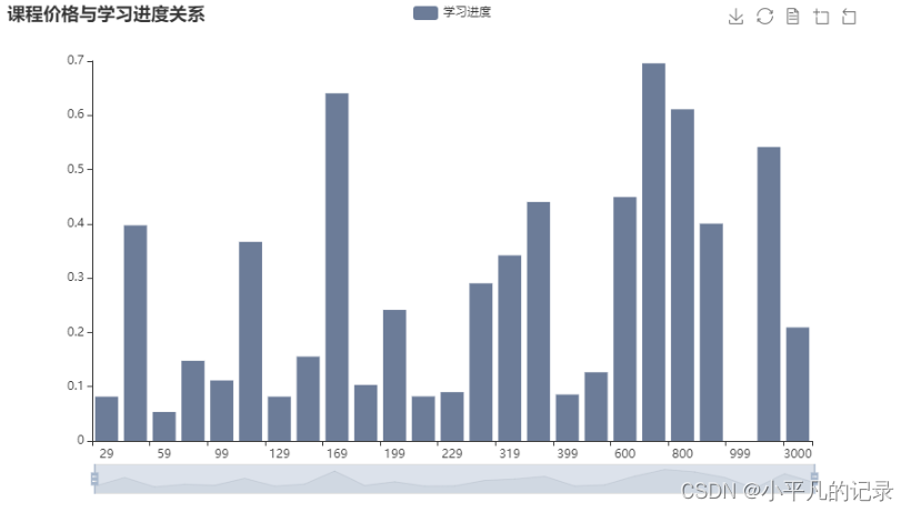
在任务 3.1 和任务 3.2 的基础上,结合用户学习进度数据,分析付费课程和免费课程的差异,给出线上课程的综合推荐策略。
study_information_shichang = study_information.groupby(by='course_id',as_index=False)['shichang'].mean()
study_information_shichang['shichang'] = study_information_shichang['shichang']/100
study_information_price = study_information.groupby(by='course_id',as_index=False)['price'].mean()
study_information_price2 = study_information_price.sort_values(by='price',ascending=True)
study_information_price2 = study_information_price2[study_information_price2['price']>0]
result = pd.merge(study_information_price2, study_information_shichang,on='course_id')
result = result.groupby(by='price',as_index=False)['shichang'].mean()
result.head()
.dataframe tbody tr th {
    vertical-align: top;
}

.dataframe thead th {
    text-align: right;
}
| price | shichang | |
|---|---|---|
| 0 | 29.0 | 0.081564 |
| 1 | 49.0 | 0.397283 |
| 2 | 59.0 | 0.053457 |
| 3 | 79.0 | 0.147661 |
| 4 | 99.0 | 0.111417 |
from pyecharts.globals import ThemeType
x_data = list(result['price'])
y_data = list(result['shichang'])

bar = (Bar()
    #init_opts=opts.InitOpts(theme=ThemeType.VINTAGE))  # 设置主题
       .add_xaxis(x_data)
       .add_yaxis('学习进度', y_data)
        .set_colors(["#6C7C98"])  # 柱子的颜色
          #.reversal_axis()   # xy轴交换
       .set_global_opts(
            title_opts=opts.TitleOpts(title="课程价格与学习进度关系"),                         # 标题
            toolbox_opts=opts.ToolboxOpts(),                                                     # 工具箱
            datazoom_opts=opts.DataZoomOpts(range_start=0,range_end=100)                         # 横轴缩放
        )
        .set_series_opts(
        # 为了不影响标记点,这里把标签关掉
        label_opts=opts.LabelOpts(is_show=False))
      )

bar.render_notebook()
数据分享链接:https://pan.baidu.com/s/1pKTbt24egIHO04rUFnNQ_w?pwd=djqi
提取码:djqi