%书上的代码，和FEM符合的更好
%在这个代码里试着把单位原胞的相对介电常数分布画出来
%这个代码的单位原胞的中心就是(0,0)点，也就是坐标原点
%The program for the computation of the PhC photonic
%band structure for 2D PhC.
%Parameters of the structure are defined by the PhC
%period, elements radius, and by the permittivities
%of elements and background material.
%Input parameters: PhC period, radius of an
%element, permittivities
%Output data: The band structure of the 2D PhC.
clear all;clc;close all
%The variable a defines the period of the structure.
%It influences on results in case of the frequency
%normalization.
a=1e-6; % in meters，晶格常数，单位m
%The variable r contains elements radius. Here it is
%defined as a part of the period.
r=0.4*a; % in meters，单位m，介质柱半径
%The variable eps1 contains the information about
%the relative background material permittivity.
eps1=9;%背景材料介电常数
%The variable eps2 contains the information about
%permittivity of the elements composing PhC. In our
%case permittivities are set to form the structure
%perforated membrane
eps2=1;%介质柱的相对介电常数
%The variable precis defines the number of k-vector
%points between high symmetry points
precis=20;%和BZ区的离散有关
%The variable nG defines the number of plane waves.
%Since the number of plane waves cannot be
%arbitrary value and should be zero-symmetric, the
%total number of plane waves may be determined
%as (nG*2-1)^2
nG=15;%和平面波的数量有关
%The variable precisStruct defines contains the
%number of nodes of discretization mesh inside in
%unit cell discretization mesh elements.
precisStruct=50;%单位原胞离散份数，最好设为偶数
%The following loop carries out the definition
%of the unit cell. The definition is being
%made in discreet form by setting values of inversed
%dielectric function to mesh nodes.
nx=1;
for countX=-a/2:a/precisStruct:a/2%就是网格节点的x坐标
ny=1;
for countY=-a/2:a/precisStruct:a/2%就是网格节点的y坐标
%The following condition allows to define the circle
%with of radius r
if(sqrt(countX^2+countY^2)<r)%判断网格节点坐标是否处于中心的介质柱内
%Setting the value of the inversed dielectric
%function to the mesh node
struct(nx,ny)=1/eps2;
%Saving the node coordinate
xSet(nx)=countX;
ySet(ny)=countY;
else
struct(nx,ny)=1/eps1;
xSet(nx)=countX;
ySet(ny)=countY;
end
ny=ny+1;
end
nx=nx+1;
end
%The computation of the area of the mesh cell. It is
%necessary for further computation of the Fourier
%expansion coefficients.
dS=(a/precisStruct)^2;%单位微元的面积
%Forming 2D arrays of nods coordinates
xMesh=meshgrid(xSet(1:length(xSet)-1));
yMesh=meshgrid(ySet(1:length(ySet)-1))';
%Transforming values of inversed dielectric function
%for the convenience of further computation
structMesh=struct(1:length(xSet)-1,...
1:length(ySet)-1)*dS/(max(xSet)-min(xSet))^2;%就是(C10)的一部分

%Defining the k-path within the Brilluoin zone. The
%k-path includes all high symmetry points and precis
%points between them
kx(1:precis+1)=0:pi/a/precis:pi/a;
ky(1:precis+1)=zeros(1,precis+1);
kx(precis+2:precis+precis+1)=pi/a;
ky(precis+2:precis+precis+1)=...
pi/a/precis:pi/a/precis:pi/a;
kx(precis+2+precis:precis+precis+1+precis)=...
pi/a-pi/a/precis:-pi/a/precis:0;
ky(precis+2+precis:precis+precis+1+precis)=...
pi/a-pi/a/precis:-pi/a/precis:0;
%After the following loop, the variable numG will
%contain real number of plane waves used in the
%Fourier expansion
numG=1;
%The following loop forms the set of reciprocal
%lattice vectors.
for Gx=-nG*2*pi/a:2*pi/a:nG*2*pi/a
for Gy=-nG*2*pi/a:2*pi/a:nG*2*pi/a
G(numG,1)=Gx;
G(numG,2)=Gy;
numG=numG+1;
end
end
%numG为82，实际上多了1
%The next loop computes the Fourier expansion
%coefficients which will be used for matrix
%differential operator computation.
for countG=1:numG-1
    Mark0=countG/(numG-1)
for countG1=1:numG-1
    temp=exp(1i*((G(countG,1)-G(countG1,1))*...
xMesh+(G(countG,2)-G(countG1,2))*yMesh));

CN2D_N(countG,countG1)=sum(sum(structMesh.*...
temp));
end
end




%The next loop computes matrix differential operator
%in case of TE mode. The computation
%is carried out for each of earlier defined
%wave vectors.
for countG=1:numG-1
     Mark=countG/(numG-1)
for countG1=1:numG-1
for countK=1:length(kx)
M(countK,countG,countG1)=...
CN2D_N(countG,countG1)*((kx(countK)+G(countG,1))*...
(kx(countK)+G(countG1,1))+...
(ky(countK)+G(countG,2))*(ky(countK)+G(countG1,2)));
end
end
end
%The computation of eigen-states is also carried
%out for all wave vectors in the k-path.
for countK=1:length(kx)
%Taking the matrix differential operator for current
%wave vector.
MM(:,:)=M(countK,:,:);
%Computing the eigen-vectors and eigen-states of
%the matrix
[D,V]=eig(MM);
%Transforming matrix eigen-states to the form of
%normalized frequency.
dispe(:,countK)=sqrt(V*ones(length(V),1))*a/2/pi;
end
%Plotting the band structure
%Creating the output field
figure(3);
%Creating axes for the band structure output.
ax1=axes;
%Setting the option
%drawing without cleaning the plot
hold on;
%Plotting the first 8 bands
for u=1:8
plot(abs(dispe(u,:)),'r','LineWidth',2);
%If there are the PBG, mark it with blue rectangle
if(min(dispe(u+1,:))>max(dispe(u,:)))
rectangle('Position',[1,max(dispe(u,:)),...
length(kx)-1,min(dispe(u+1,:))-...
max(dispe(u,:))],'FaceColor','b',...
'EdgeColor','b');
end
end
%Signing Labeling the axes
%下面是和FEM算的数据比较，没有的话可以删除下面这段%%
Data=csvread('C:\Users\LUO1\Desktop\ComsolDate.csv');
uniX=unique(Data(:,1));
Ymat=[];
for zz=1:length(uniX)
    Ymat=[Ymat,Data(Data(:,1)==uniX(zz),2)];    
end
plot(1:size(Ymat,2),Ymat,'bo','MarkerSize',3)
%%%%%绘制FEM的数据%%%%%%%

set(ax1,'xtick',...
[1 precis+1 2*precis+1 3*precis+1]);
set(ax1,'xticklabel',['G';'X';'M';'G']);
ylabel('Frequency \omegaa/2\pic','FontSize',16);
xlabel('Wavevector','FontSize',16);
xlim([1 length(kx)])
set(ax1,'XGrid','on');
 title('book')

在这里插入图片描述
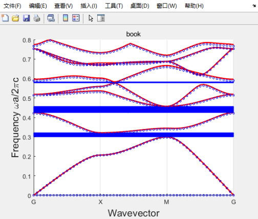
蓝色小圆是FEM绘制的能带。我原先按照自己的理解改动了下上面的代码，但是和FEM的结果符合得没上面的代码好。

抄的书上的代码: Photonic Crystals Physics and Practical Modeling (Igor A. Sukhoivanov, Igor V. Guryev (auth.))

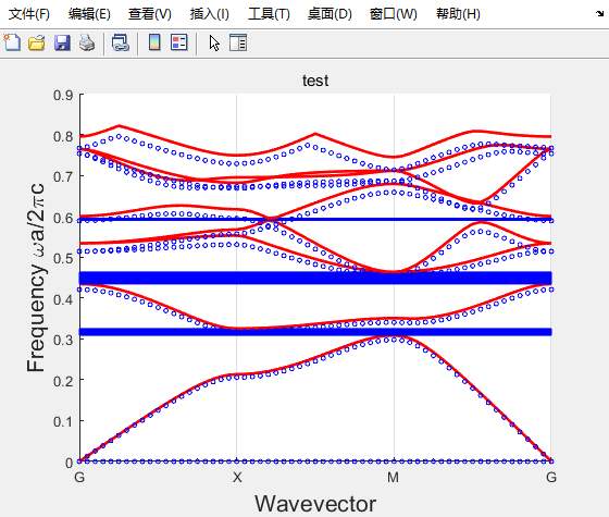
下面是相同参数，但按照我自己的理解改了一点点的代码，结果和FEM的结果符合得不是很好，有无这方面的大佬评论区解释下原因？或者任何见解也行

%这份代码和FEM符合的不是很好
%在这个代码里试着把单位原胞的相对介电常数分布画出来
%这个代码的单位原胞的中心就是(0,0)点，也就是坐标原点
%The program for the computation of the PhC photonic
%band structure for 2D PhC.
%Parameters of the structure are defined by the PhC
%period, elements radius, and by the permittivities
%of elements and background material.
%Input parameters: PhC period, radius of an
%element, permittivities
%Output data: The band structure of the 2D PhC.
clear all;clc;close all
%The variable a defines the period of the structure.
%It influences on results in case of the frequency
%normalization.
a=1e-6; % in meters，晶格常数，单位m
%The variable r contains elements radius. Here it is
%defined as a part of the period.
r=0.4*a; % in meters，单位m，介质柱半径
%The variable eps1 contains the information about
%the relative background material permittivity.
eps1=9;%背景材料介电常数
%The variable eps2 contains the information about
%permittivity of the elements composing PhC. In our
%case permittivities are set to form the structure
%perforated membrane
eps2=1;%介质柱的相对介电常数
%The variable precis defines the number of k-vector
%points between high symmetry points
precis=20;%和BZ区的离散有关
%The variable nG defines the number of plane waves.
%Since the number of plane waves cannot be
%arbitrary value and should be zero-symmetric, the
%total number of plane waves may be determined
%as (nG*2-1)^2
nG=15;%和平面波的数量有关
%The variable precisStruct defines contains the
%number of nodes of discretization mesh inside in
%unit cell discretization mesh elements.
precisStruct=50;%单位原胞离散份数，最好设为偶数
%The following loop carries out the definition
%of the unit cell. The definition is being
%made in discreet form by setting values of inversed
%dielectric function to mesh nodes.
nx=1;
for countX=-a/2:a/precisStruct:a/2%就是网格节点的x坐标
ny=1;
for countY=-a/2:a/precisStruct:a/2%就是网格节点的y坐标
%The following condition allows to define the circle
%with of radius r
if(sqrt(countX^2+countY^2)<r)%判断网格节点坐标是否处于中心的介质柱内
%Setting the value of the inversed dielectric
%function to the mesh node
struct(nx,ny)=1/eps2;
%Saving the node coordinate
xSet(nx)=countX;
ySet(ny)=countY;
else
struct(nx,ny)=1/eps1;
xSet(nx)=countX;
ySet(ny)=countY;
end
ny=ny+1;
end
nx=nx+1;
end
%The computation of the area of the mesh cell. It is
%necessary for further computation of the Fourier
%expansion coefficients.
dS=(a/precisStruct)^2;%单位微元的面积
%Forming 2D arrays of nods coordinates
xMesh=meshgrid(xSet(1:length(xSet)));
yMesh=meshgrid(ySet(1:length(ySet)))';
%Transforming values of inversed dielectric function
%for the convenience of further computation
structMesh=struct(1:length(xSet),...
1:length(ySet))*dS/(max(xSet)-min(xSet))^2;%就是(C10)的一部分

%Defining the k-path within the Brilluoin zone. The
%k-path includes all high symmetry points and precis
%points between them
kx(1:precis+1)=0:pi/a/precis:pi/a;
ky(1:precis+1)=zeros(1,precis+1);
kx(precis+2:precis+precis+1)=pi/a;
ky(precis+2:precis+precis+1)=...
pi/a/precis:pi/a/precis:pi/a;
kx(precis+2+precis:precis+precis+1+precis)=...
pi/a-pi/a/precis:-pi/a/precis:0;
ky(precis+2+precis:precis+precis+1+precis)=...
pi/a-pi/a/precis:-pi/a/precis:0;
%After the following loop, the variable numG will
%contain real number of plane waves used in the
%Fourier expansion
numG=1;
%The following loop forms the set of reciprocal
%lattice vectors.
for Gx=-nG*2*pi/a:2*pi/a:nG*2*pi/a
for Gy=-nG*2*pi/a:2*pi/a:nG*2*pi/a
G(numG,1)=Gx;
G(numG,2)=Gy;
numG=numG+1;
end
end
%numG为82，实际上多了1
%The next loop computes the Fourier expansion
%coefficients which will be used for matrix
%differential operator computation.
for countG=1:numG-1
    Mark0=countG/(numG-1)
for countG1=1:numG-1
    temp=exp(1i*((G(countG,1)-G(countG1,1))*...
xMesh+(G(countG,2)-G(countG1,2))*yMesh));

CN2D_N(countG,countG1)=sum(sum(structMesh.*...
temp));
end
end




%The next loop computes matrix differential operator
%in case of TE mode. The computation
%is carried out for each of earlier defined
%wave vectors.
for countG=1:numG-1
    Mark=countG/(numG-1)
for countG1=1:numG-1
for countK=1:length(kx)
M(countK,countG,countG1)=...
CN2D_N(countG,countG1)*((kx(countK)+G(countG,1))*...
(kx(countK)+G(countG1,1))+...
(ky(countK)+G(countG,2))*(ky(countK)+G(countG1,2)));
end
end
end
%The computation of eigen-states is also carried
%out for all wave vectors in the k-path.
for countK=1:length(kx)
%Taking the matrix differential operator for current
%wave vector.
MM(:,:)=M(countK,:,:);
%Computing the eigen-vectors and eigen-states of
%the matrix
[D,V]=eig(MM);
%Transforming matrix eigen-states to the form of
%normalized frequency.
dispe(:,countK)=sqrt(V*ones(length(V),1))*a/2/pi;
end
%Plotting the band structure
%Creating the output field
figure(3);
%Creating axes for the band structure output.
ax1=axes;
%Setting the option
%drawing without cleaning the plot
hold on;
%Plotting the first 8 bands
for u=1:8
plot(abs(dispe(u,:)),'r','LineWidth',2);
%If there are the PBG, mark it with blue rectangle
if(min(dispe(u+1,:))>max(dispe(u,:)))
rectangle('Position',[1,max(dispe(u,:)),...
length(kx)-1,min(dispe(u+1,:))-...
max(dispe(u,:))],'FaceColor','b',...
'EdgeColor','b');
end
end
Data=csvread('C:\Users\LUO1\Desktop\ComsolDate.csv');
uniX=unique(Data(:,1));
Ymat=[];
for zz=1:length(uniX)
    Ymat=[Ymat,Data(Data(:,1)==uniX(zz),2)];    
end
plot(1:size(Ymat,2),Ymat,'bo','MarkerSize',3)
%Signing Labeling the axes
set(ax1,'xtick',...
[1 precis+1 2*precis+1 3*precis+1]);
set(ax1,'xticklabel',['G';'X';'M';'G']);
ylabel('Frequency \omegaa/2\pic','FontSize',16);
xlabel('Wavevector','FontSize',16);
xlim([1 length(kx)])
set(ax1,'XGrid','on');
 title('test')

和FEM的对比：
在这里插入图片描述

%================================================%
我明白为什么我改动后的代码是错的了，原因是需要把xMesh、yMesh当作每个离散小微元的中心坐标，所以书上的代码更准确。

上面的理解又是错的，书上代码参考的那个数值求傅里叶系数的公式应该理解成二维离散傅里叶变换(2D DFT)，总之这个知识点的却非常细微，不注意很容易以为自己搞懂了，但实际上理解是错的。

%=======================================%
为何下面两段代码的结果之差不是严格等于0？非常奇怪。有无这方面的大佬解释下？

Kappa(countG,countG1)*...
 (norm([kx(countK)+G(countG,1),ky(countK)+G(countG,2)])*...
 norm([kx(countK)+G(countG1,1),ky(countK)+G(countG1,2)]))

Kappa(countG,countG1)*...
norm([kx(countK)+G(countG,1),ky(countK)+G(countG,2)])*...
norm([kx(countK)+G(countG1,1),ky(countK)+G(countG1,2)])

写PWEM算法的时候只有用第一段代码得到的结果才是对的。
%=======================================%

%=========================================%
在某些nG参数下，书上代码绘制的能带会全部挤到0附近不知道为何，
但是如果加大precisStruct结果又会变回正常；在使用数值方法计算相对介电函数的傅里叶系数时nG和precisStruct参数的相对大小需要小心设置

后面我找到了这一现象可能的原因，和离散傅里叶变换(DFT)，离散傅里叶级数(DFS)的公式具体形式有关。基于此我猜测有关系：2*nG+1应小于或等于precisStruct

%=========================================%

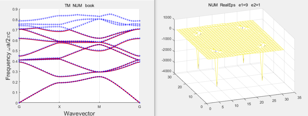
对书上代码的改写(TE、TM都可以计算，数值或解析方法算相对介电函数的傅里叶系数)

实际上无论算TE 还是TM能带数值方法算的相对介电函数的傅里叶系数得到的能带反而比解析方法得到的能带和FEM方法误差更小（实际上解析方法算的相对介电函数比数值方法的质量好些），不清楚为何会这样。
图像如下：
在这里插入图片描述

代码：

%为什么按照我的想法去设置微元的中心坐标效果不行？
%数值法算Kappa的结果和FEM更接近，不知道为何
clear ;clc;close all
TEorTM='TM';
NUMorANA='ANA';%数值或解析方法算Kappa矩阵(傅里叶系数)
a=1e-6; % in meters，晶格常数，单位m

r=0.4*a; % in meters，单位m，介质柱半径

eps1=9;%背景材料介电常数

eps2=1;%介质柱的相对介电常数

precis=20;%和BZ区的离散有关

nG=16;%和平面波的数量有关

precisStruct=44;%单位原胞离散段数(x、y方向)，最好设为偶数，
%因此节点数为precisStruct+1

%%%正空间基矢(可自己设置)%%%
a1=[a,0,0];%为方便求倒格子基矢，必须是三维矢量
a2=[0,a,0];
%%%正空间基矢%%%%%%%%%

%%%%求倒格子基矢%%%%%
a3=[0,0,1];%单位向量
Omega=abs(a3*cross(a1,a2)');%正空间单位原胞面积
s=2*pi./Omega;
b1(1,1)=a2(1,2);b1(1,2)=-a2(1,1);
b2(1,1)=-a1(1,2);b2(1,2)=a1(1,1);
b1=b1.*s;%行数组，最终结果(必须是行数组)
b2=b2.*s;%行数组，最终结果(必须是行数组)
%%%%求倒格子基矢%%%%%



nodeSet=-a/2:a/precisStruct:a/2;
len_nodeSet=length(nodeSet);
%初始化
struct=zeros(len_nodeSet,len_nodeSet);
xMesh0=zeros(len_nodeSet,len_nodeSet);
yMesh0=zeros(len_nodeSet,len_nodeSet);

for nx=1:len_nodeSet
    countX=nodeSet(nx);
    for ny=1:len_nodeSet
        
        countY=nodeSet(ny);
        if(sqrt(countX^2+countY^2)<r)%判断网格节点坐标是否处于中心的介质柱内
            
            struct(nx,ny)=1/eps2;%其实就是每个节点的相对介电常数
            xMesh0(nx,ny)=countX;%其实就是每个节点的x坐标
            yMesh0(nx,ny)=countY;%其实就是每个节点的y坐标
        else
            struct(nx,ny)=1/eps1;
            xMesh0(nx,ny)=countX;
            yMesh0(nx,ny)=countY;
        end
        
    end
    
end
xMesh0(:,end)=[];
xMesh0(end,:)=[];
yMesh0(:,end)=[];
yMesh0(end,:)=[];

%其实xSet=ySet=[-a/2:a/precisStruct:a/2]


dS=(a/precisStruct)^2;%单位微元的面积
%Forming 2D arrays of nods coordinates

%注意xMesh=xMesh0.'
%注意yMesh=yMesh0.'
%注意xMesh=yMesh0
%注意yMesh=xMesh0
%xMesh0、yMesh0其实是节点的坐标？
%=======================%
%=======================%
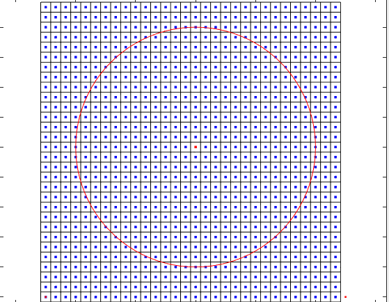
figure
for ii = 1:numel(xMesh0)
    plot(xMesh0(ii),yMesh0(ii),'b.','Markersize',8)
    hold on
    
    rectangle('Position',[xMesh0(ii)-0.5*(a/precisStruct),...
        yMesh0(ii)-0.5*(a/precisStruct),(a/precisStruct),(a/precisStruct)]);
    
end
xx1=a/2;
siteSto=[xx1,xx1;xx1,-xx1;-xx1,xx1;-xx1,-xx1];
hold on
scatter(siteSto(:,1),siteSto(:,2),'r.')
hold on
plot(0,0,'r.','Markersize',8)
hold on
% x y是中心，r是半径
rectangle('Position',[0-r,0-r,2*r,2*r],'Curvature',[1,1],'edgecolor',[1,0,0])
hold off
axis equal
title('xMesh、yMesh')
%=======================%
%=======================%

structMesh=struct(1:precisStruct,...
    1:precisStruct)*dS/Omega;%就是公式(C10)的一部分
%注意struct(1:length(xSet)-1,1:length(ySet)-1)等价于
%struct(:,end)=[];struct(end,:)=[];

%========离散不可约布里渊区(只适用于正方晶格)==========%
kx(1:precis+1)=0:pi/a/precis:pi/a;
ky(1:precis+1)=zeros(1,precis+1);
kx(precis+2:precis+precis+1)=pi/a;
ky(precis+2:precis+precis+1)=...
    pi/a/precis:pi/a/precis:pi/a;
kx(precis+2+precis:precis+precis+1+precis)=...
    pi/a-pi/a/precis:-pi/a/precis:0;
ky(precis+2+precis:precis+precis+1+precis)=...
    pi/a-pi/a/precis:-pi/a/precis:0;

%========离散不可约布里渊区(只适用于正方晶格)==========%


%The following loop forms the set of reciprocal
%lattice vectors.
G=zeros((2*nG+1)^2,2);
numG=0;
for m=-nG:nG
    for n=-nG:nG
        numG=numG+1;
        
        G(numG,1:2)=m.*b1+n.*b2;
        
    end
end
%G里面没有重复的G_{||}向量
numG=size(G,1);
%The next loop computes the Fourier expansion
%coefficients which will be used for matrix
%differential operator computation.
%遍历G数组

Kappa=zeros(numG,numG);
Indexset=-nG:nG;
if strcmp(NUMorANA,'NUM')==1%数值法计算Kappa
    
    for countG=1:numG
        Mark0=countG/(numG)
        for countG1=1:numG
            
            temp=exp(-1i*((G(countG,1)-G(countG1,1)).*...
                xMesh0+(G(countG,2)-G(countG1,2)).*yMesh0));%矩阵
            
            Kappa(countG,countG1)=sum(sum(structMesh.*...
                temp));%其实就是kappa(G_{||}-G_{||}^{\prime}})构成的矩阵
            %G(countG,1:2)其实就是G_{||}，
            %G(countG1,1:2)其实就是G_{||}^{\prime}
            
            
        end
    end
    
    %%%%%%%%计算kappa(G_{||})%%%%%%%%
    Gmat=zeros(length(Indexset),length(Indexset));
    Kapmat=zeros(length(Indexset),length(Indexset));
    for m=1:length(Indexset)
        for n=1:length(Indexset)
            g0=Indexset(m).*b1+Indexset(n).*b2;%行数组
            Gmat(m,n)=g0(1)+1j.*g0(2);
            
            temp=exp(-1i*(g0(1).*...
                xMesh0+g0(2).*yMesh0));%矩阵
            
            Kapmat(m,n)=sum(sum(structMesh.*...
                temp));
         
        end
    end
    %%%%%%%%%%%%%%%%%%%%%%%
    
    
    
end


f=(pi*r^2)/Omega;
if strcmp(NUMorANA,'ANA')==1%解析法计算Kappa
    
    for countG=1:numG
        Mark0=countG/(numG)
        for countG1=1:numG
            temp=norm(G(countG,1:2)-G(countG1,1:2))*r;%|G|r
            
            if temp==0
                Kappa(countG,countG1)=1/eps1+f*(1/eps2-1/eps1);
            else
                Kappa(countG,countG1)=2*f*(1/eps2-1/eps1)*besselj(1,temp)/temp;
            end
            
            
            %其实就是kappa(G_{||}-G_{||}^{\prime}})构成的矩阵
            %G(countG,1:2)其实就是G_{||}，
            %G(countG1,1:2)其实就是G_{||}^{\prime}
        end
    end
    
      %%%%%%%%计算kappa(G_{||})%%%%%%%%
    Gmat=zeros(length(Indexset),length(Indexset));
    Kapmat=zeros(length(Indexset),length(Indexset));
    for m=1:length(Indexset)
        for n=1:length(Indexset)
            g0=Indexset(m).*b1+Indexset(n).*b2;%行数组
            normG=norm(g0);%|G|
            Gmat(m,n)=g0(1)+1j.*g0(2);
            
            if Indexset(m)==0 && Indexset(n)==0
                Kapmat(m,n)=1/eps1+f*(1/eps2-1/eps1);
            else
                Kapmat(m,n)=2*f*(1/eps2-1/eps1)*besselj(1,(normG*r))/(normG*r);
            end
        
        end
    end
    %%%%%%%%%%%%%%%%%%%%%%%
    
    
end


%======绘制Kappa(G_{||})还原的相对介电常数分布==========%
%G_{||}-G_{||}^{\prime}}包含了很多重复元素
%因此kappa(G_{||}-G_{||}^{\prime}})不能用来恢复相对介电常数
%分布,只能用kappa(G_{||})
EpsMat=zeros(precisStruct+1,precisStruct+1);
for uu=1:precisStruct+1
    uu/(precisStruct+1)
    X=nodeSet(uu);
    for vv=1:precisStruct+1
        Y=nodeSet(vv);
        EpsMat(uu,vv)=sum(sum(Kapmat.*exp(1j*(X.*real(Gmat)+Y.*imag(Gmat)))));
        
    end
end
figure
mesh(1./real(EpsMat)) %画图
title([NUMorANA,'  RealEps','   e1=',num2str(eps1),'   e2=',num2str(eps2)])

figure
mesh(1./imag(EpsMat)) %画图
title([NUMorANA,'  ImagEps','   e1=',num2str(eps1),'   e2=',num2str(eps2)])

figure
imagesc(1./real(EpsMat))
colorbar


%======绘制Kappa(G_{||})还原的相对介电常数分布==========%

%构建特征矩阵

M=zeros(numG,numG,length(kx));%特征矩阵初始化
for countK=1:length(kx)
    Mark=countK/length(kx)
    for countG=1:numG
        for countG1=1:numG
            
            if strcmp(TEorTM,'TE')==1%TE
                M(countG,countG1,countK)=...
                    Kappa(countG,countG1)*...
                    ([kx(countK)+G(countG,1),ky(countK)+G(countG,2)]*...
                    ([kx(countK)+G(countG1,1),ky(countK)+G(countG1,2)].'));
            end
            
            if strcmp(TEorTM,'TM')==1%TM
                M(countG,countG1,countK)=...
                    Kappa(countG,countG1)*...
                    (norm([kx(countK)+G(countG,1),ky(countK)+G(countG,2)])*...
                    norm([kx(countK)+G(countG1,1),ky(countK)+G(countG1,2)]));
            end
            
            
        end
    end
end

%The computation of eigen-states is also carried
%out for all wave vectors in the k-path.
for countK=1:length(kx)
    %Taking the matrix differential operator for current
    %wave vector.
    MM(:,:)=M(:,:,countK);
    %Computing the eigen-vectors and eigen-states of
    %the matrix
    [D,V]=eig(MM);
    %Transforming matrix eigen-states to the form of
    %normalized frequency.
    dispe(:,countK)=sqrt(V*ones(length(V),1))*a/2/pi;
end
%Plotting the band structure
%Creating the output field
figure;
%Creating axes for the band structure output.
ax1=axes;
%Setting the option
%drawing without cleaning the plot
hold on;
%Plotting the first 8 bands
for u=1:8
    plot(abs(dispe(u,:)),'r','LineWidth',2);
    %If there are the PBG, mark it with blue rectangle
    if(min(dispe(u+1,:))>max(dispe(u,:)))
        rectangle('Position',[1,max(dispe(u,:)),...
            length(kx)-1,min(dispe(u+1,:))-...
            max(dispe(u,:))],'FaceColor','b',...
            'EdgeColor','b');
    end
end
%Signing Labeling the axes
%下面是和FEM算的数据比较，没有的话可以删除下面这段%%
if strcmp(TEorTM,'TE')==1
    Data=csvread('C:\Users\LUO1\Desktop\ComsolDateTE.csv');
end
if strcmp(TEorTM,'TM')==1
    Data=csvread('C:\Users\LUO1\Desktop\ComsolDateTM.csv');
end

uniX=unique(Data(:,1));
Ymat=[];
for zz=1:length(uniX)
    Ymat=[Ymat,Data(Data(:,1)==uniX(zz),2)];
end

plot(1:size(Ymat,2),Ymat,'bo','MarkerSize',3)
hold off
%%%%%绘制FEM的数据%%%%%%%

set(ax1,'xtick',...
    [1 precis+1 2*precis+1 3*precis+1]);
set(ax1,'xticklabel',['G';'X';'M';'G']);
ylabel('Frequency \omegaa/2\pic','FontSize',16);
xlabel('Wavevector','FontSize',16);
xlim([1 length(kx)])
set(ax1,'XGrid','on');
title([TEorTM,'  ',NUMorANA,'   book'])