💥💥💞💞欢迎来到本博客❤️❤️💥💥
🏆博主优势:🌞🌞🌞博客内容尽量做到思维缜密,逻辑清晰,为了方便读者。
⛳️座右铭:行百里者,半于九十。
📋📋📋本文目录如下:🎁🎁🎁
目录
💥1 概述
📚2 运行结果
🎉3 参考文献
🌈4 Matlab代码实现
💥1 概述
随机规划的三个分支分别为期望值模型、机会约束规划和相关机会规划。机会约束规划是继期望值模型之后,由A. Charnes和 W.W. Cooper于 1959年提出的第二类随机规划[33]。CCP是考虑到所做决策在不利情况发生时可能不满足约束条件而采用的一种原则:即允许所做决策在一定程度上不满足约束条件,但该决策使约束条件成立的概率不小于某一置信水平。一般形式的机会约束可表示为:
CCP 是处理随机规划问题的经典方法之一,其主要利用概率形式约束处理约束条件中含有随机变量的优化问题,CCP 方法具有以下特点:
(1)为了有效处理含随机变量的约束问题,CCP 将传统规划模型中的硬约束变为概率形式约束,以实现考虑随机变量的大概率事件,减小低概率极端事件对最优解的影响,一定程度上提高了最优解的合理性。
(2)对于问题中的随机变量,仅在约束中以机会约束的形式进行体现,未在目标函数中予以反映,而规划问题的最优解与概率约束的置信水平直接相关,且其置信水平可根据决策者的风险偏好或实际经验进行设定。
(3)当模型中含有多个机会约束时,在优化过程中将予以同等对待,无主次顺序之分。
(4)CCP 模型的求解过程中常需利用 MCS 过程和智能算法,其求解过程较为复杂,求解效率与结果质量都受到一定影响;若通过解析法求解则需较复杂的数学推导,以上因素在一定程度上了限制了 CCP 方法在复杂问题中的应用。
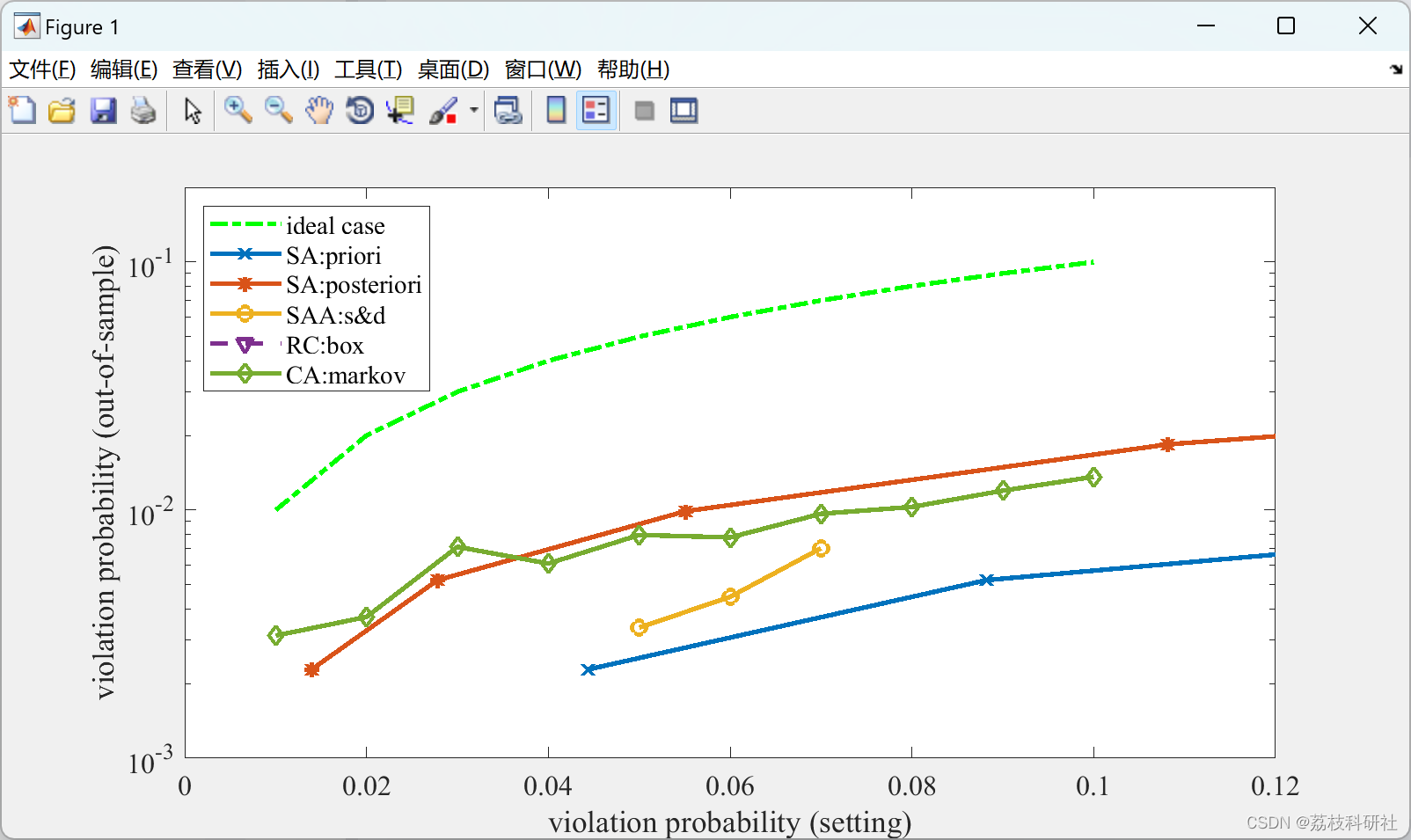
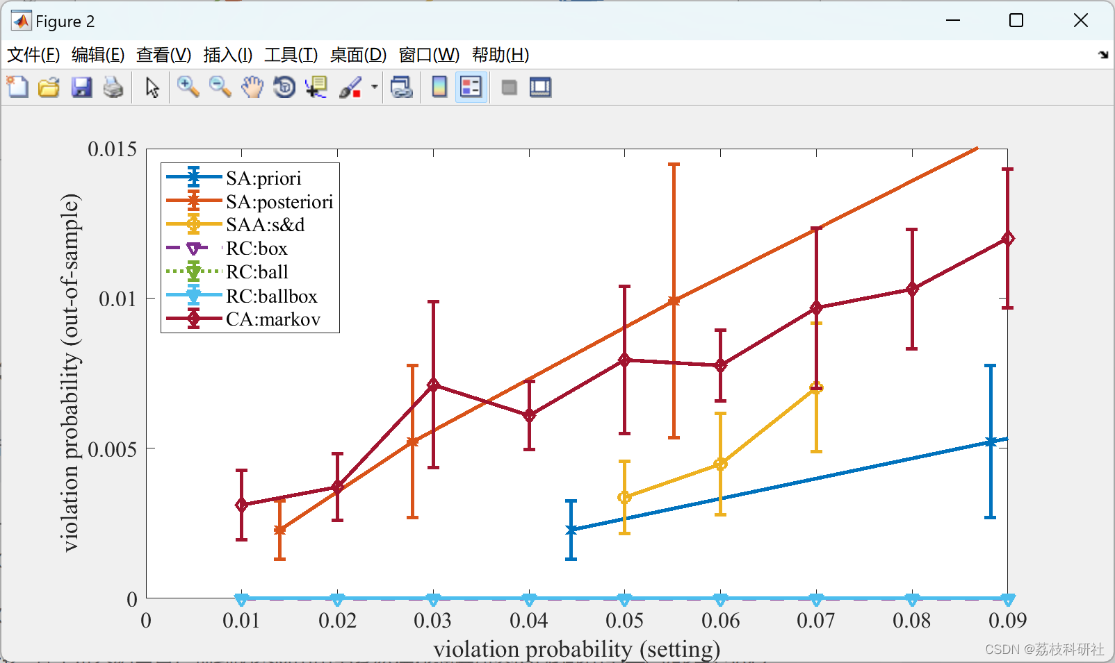
📚2 运行结果
部分代码:
clear; clc; close all;
fig_size = [10,10,800,400];
beta = 10^(-2);
% casename = 'ex_case3sc'; N = 100;
casename = 'ex_case24_ieee_rts'; N = 2048;
eps_scale = 0.01:0.01:0.1;
result_sa = load([casename,'-scenario approach-results.mat']);
result_ca = load([casename,'-convex approximation-type-results-N=',num2str(N),'.mat']);
result_saa = load([casename,'-sample average approximation-sampling and discarding-results-N=',num2str(N),'.mat']);
result_rc = load([casename,'-robust counterpart-results-N=',num2str(N),'.mat']);
% result_lb = load([casename,'-obj-lower-bound.mat']);
f_eps = figure('Position', fig_size);
lgd_str = {};
plot(eps_scale,eps_scale,'g-.','LineWidth',2), hold on, lgd_str = [lgd_str,'ideal case'];
plot(nanmean(result_sa.eps_pri,2), nanmean(result_sa.eps_empirical,2),'-x','LineWidth',2), hold on, lgd_str = [lgd_str,'SA:priori'];
plot(nanmean(result_sa.eps_post,2), nanmean(result_sa.eps_empirical,2),'-*','LineWidth',2), hold on, lgd_str = [lgd_str,'SA:posteriori'];
plot(result_saa.epsilons, nanmean(result_saa.eps_empirical,2),'-o','LineWidth',2), hold on, lgd_str = [lgd_str,'SAA:s&d'];
plot(result_rc.eps, nanmean(result_rc.eps_empirical_box,2)*ones(size(result_rc.eps)),'--v','LineWidth',2), hold on, lgd_str = [lgd_str,'RC:box'];
% plot(result_rc.eps, nanmean(result_rc.eps_empirical_ball,2),':v','LineWidth',2), hold on, lgd_str = [lgd_str,'RC:ball'];
% plot(result_rc.eps, nanmean(result_rc.eps_empirical_ballbox,2),'-v','LineWidth',2), hold on, lgd_str = [lgd_str,'RC:ballbox'];
% plot(result_rc.eps, nanmean(result_rc.eps_empirical_budget,2),'-.v','LineWidth',2), hold on, lgd_str = [lgd_str,'RC:budget'];
plot(result_ca.eps, nanmean(result_ca.eps_empirical,2),'-d','LineWidth',2), hold on, lgd_str = [lgd_str,'CA:markov'];
legend(lgd_str,'Location','NorthWest')
set(gca,'yscale','log')
% xlim([0,0.9]), ylim([1e-4 10])
xlim([0,0.12]), ylim([1e-3 0.2])
xlabel('violation probability (setting)'),ylabel('violation probability (out-of-sample)')
set(gca,'FontSize',12,'fontname','times')
print(f_eps,'-depsc','-painters',[casename,'-all-methods-epsilon.eps'])
f_eps_err = figure('Position', fig_size);
lgd_str = {};
% plot(eps_scale,eps_scale,'g-.','LineWidth',2), hold on, lgd_str = [lgd_str,'ideal case'];
errorbar(nanmean(result_sa.eps_pri,2), nanmean(result_sa.eps_empirical,2),nanstd(result_sa.eps_empirical,[],2),'-x','LineWidth',2), hold on, lgd_str = [lgd_str,'SA:priori'];
errorbar(nanmean(result_sa.eps_post,2), nanmean(result_sa.eps_empirical,2),nanstd(result_sa.eps_empirical,[],2),'-*','LineWidth',2), hold on, lgd_str = [lgd_str,'SA:posteriori'];
errorbar(result_saa.epsilons, nanmean(result_saa.eps_empirical,2),nanstd(result_saa.eps_empirical,[],2),'-o','LineWidth',2), hold on, lgd_str = [lgd_str,'SAA:s&d'];
plot(result_rc.eps, nanmean(result_rc.eps_empirical_box,2)*ones(size(result_rc.eps)),'--v','LineWidth',2), hold on, lgd_str = [lgd_str,'RC:box'];
errorbar(result_rc.eps, nanmean(result_rc.eps_empirical_ball,2),nanstd(result_rc.eps_empirical_ball,[],2),':v','LineWidth',2), hold on, lgd_str = [lgd_str,'RC:ball'];
errorbar(result_rc.eps, nanmean(result_rc.eps_empirical_ballbox,2),nanstd(result_rc.eps_empirical_ballbox,[],2),'-v','LineWidth',2), hold on, lgd_str = [lgd_str,'RC:ballbox'];
% errorbar(result_rc.eps, nanmean(result_rc.eps_empirical_budget,2),nanstd(result_rc.eps_empirical_budget,[],2),'-.v','LineWidth',2), hold on,
errorbar(result_ca.eps, nanmean(result_ca.eps_empirical,2), nanstd(result_ca.eps_empirical,[],2),'-d','LineWidth',2), hold on, lgd_str = [lgd_str,'CA:markov'];
legend(lgd_str,'Location','NorthWest')
% xlim([0,0.12])
xlim([0,0.09])
% ylim([0,0.09])
xlabel('violation probability (setting)'),ylabel('violation probability (out-of-sample)')
set(gca,'FontSize',12,'fontname','times')
print(f_eps_err,'-depsc','-painters',[casename,'-all-methods-epsilon-errorbar.eps'])
f_obj = figure('Position', fig_size);
lgd_str = {};
% plot(result_lb.epsilons, result_lb.obj_low, ':^'), hold on,
% plot(nanmean(result_sa.eps_pri,2), nanmean(result_sa.obj,2),'-x','LineWidth',2), hold on, lgd_str = [lgd_str,'SA:priori'];
% plot(nanmean(result_sa.eps_post,2), nanmean(result_sa.obj,2),'-*','LineWidth',2), hold on, lgd_str = [lgd_str,'SA:posteriori'];
% plot(result_saa.epsilons, nanmean(result_saa.obj,2),'-o','LineWidth',2), hold on, lgd_str = [lgd_str,'SAA:s&d'];
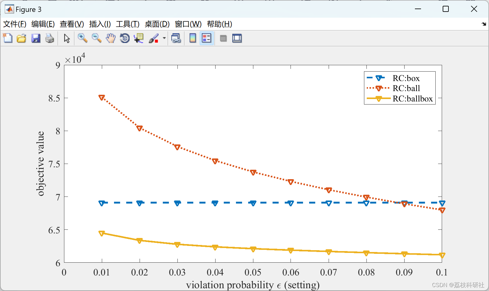
plot(result_rc.eps, nanmean(result_rc.obj_box,2)*ones(size(result_rc.eps)),'--v','LineWidth',2), hold on, lgd_str = [lgd_str,'RC:box'];
plot(result_rc.eps, nanmean(result_rc.obj_ball,2),':v','LineWidth',2), hold on, lgd_str = [lgd_str,'RC:ball'];
plot(result_rc.eps, nanmean(result_rc.obj_ballbox,2),'-v','LineWidth',2), hold on, lgd_str = [lgd_str,'RC:ballbox'];
% plot(result_rc.eps, nanmean(result_rc.obj_budget,2),'-.v','LineWidth',2), hold on,
% plot(result_ca.eps, nanmean(result_ca.obj, 2),'-d','LineWidth',2), hold on, lgd_str = [lgd_str,'CA:markov'];
legend(lgd_str)
xlabel('violation probability \epsilon (setting)'),ylabel('objective value')
xlim([0 0.1])
set(gca,'FontSize',12,'fontname','times')
print(f_obj,'-depsc','-painters',[casename,'-all-methods-objective.eps'])
% f_obj_emp = figure('Position', fig_size);
% % plot(result_lb.epsilons, result_lb.obj_low,'-^'), hold on,
% [result_sa_eps_empirical,indices] = sort( nanmean(result_sa.eps_empirical,2),'ascend' );
% plot(result_sa_eps_empirical, nanmean(result_sa.obj(indices,:),2),'-v'), hold on,
% [result_saa_eps_empirical,indices] = sort( nanmean(result_saa.eps_empirical,2),'ascend' );
% plot(result_saa_eps_empirical, nanmean(result_saa.obj(indices,:),2),'-d'), hold on,
% [result_rc_eps_empirical_box,indices] = sort( nanmean(result_rc.eps_empirical_box,2),'ascend' );
% plot(result_rc_eps_empirical_box, nanmean(result_rc.obj_box(indices,:),2),'-*'), hold on,
% [result_rc_eps_empirical_ball,indices] = sort( nanmean(result_rc.eps_empirical_ball,2),'ascend' );
% plot(result_rc_eps_empirical_ball, nanmean(result_rc.obj_ball(indices,:),2),'-*'), hold on,
% [result_rc_eps_empirical_ballbox,indices] = sort( nanmean(result_rc.eps_empirical_ballbox,2),'ascend' );
% plot(result_rc_eps_empirical_ballbox, nanmean(result_rc.obj_ballbox(indices,:),2),'-x'), hold on,
% [result_rc_eps_empirical_budget,indices] = sort( nanmean(result_rc.eps_empirical_budget,2),'ascend' );
% plot(result_rc_eps_empirical_budget, nanmean(result_rc.obj_budget(indices,:),2),'-x'), hold on,
% [result_ca_eps_empirical,indices] = sort( nanmean(result_ca.eps_empirical,2),'ascend' );
% plot(result_ca_eps_empirical, nanmean(result_ca.obj,2),'-d','LineWidth',2), hold on,
% % legend('lower bound','SA','SAA:s&d','RC:box','RC:ball','RC:ballbox','RC:budget')
% legend('SA','SAA:s&d','RC:box','RC:ball','RC:ballbox','RC:budget','CA:markov')
% set(gca,'xscale','log')
% xlim([0 0.06])
🎉3 参考文献
部分理论来源于网络,如有侵权请联系删除。
[1]付波,邓竞成,康毅恒.基于机会约束的园区综合能源系统优化调度[J].湖北工业大学学报,2023,38(01):11-14+32.
[2]耿晓路. 分布鲁棒机会约束优化问题的研究[D].湘潭大学,2018.
[3]王扬. 基于机会约束目标规划的含风电电力系统优化调度研究[D].华北电力大学(北京),2017.