R语言在RNA-seq中的应用

文章目录

R语言在RNA-seq中的应用
- 生成工作流环境
- 读取和处理数据
- - 由targets文件提供实验定义
  - 对实验数据进行质量过滤和修剪
  - 生成FASTQ质量报告
- 比对
- - 建立HISAT2索引并比对
- 读长量化
- - 读段计数
  - 样本间的相关性分析
- 差异表达分析
- - 运行edgeR
  - 可视化差异表达结果
  - 计算和绘制差异表达基因（DEG）集合的Venn图
- GO富集分析
- - 准备工作
  - 批量进行GO富集分析
  - 绘制批量GO富集分析的结果
- 层次聚类和热图绘制

生成工作流环境

之后代码运行可能会有网络问题，通过set_config函数设置即可。

.libPaths("D:/000大三下/R语言/实验/Lab4/lab4packages")
library(httr)
set_config(
  use_proxy(url="127.0.0.1", port=7890)
)
library(systemPipeR)
library(systemPipeRdata)
#####################################################
## 1. Generate workflow environment
#####################################################
setwd(choose.dir())
genWorkenvir(workflow = "rnaseq")
setwd("rnaseq")

读取和处理数据

由targets文件提供实验定义

读取和预处理实验数据。具体步骤如下：

首先，使用system.file函数找到targets.txt文件的路径，这个文件包含了所有的FASTQ文件和样本比较的信息。
然后，使用read.delim函数读取targets.txt文件，忽略以#开头的注释行，并只保留前四列。
最后，打印出targets对象，查看数据的结构和内容。

## 2. Read preprocessing
#####################################################
## 2.1 Experiment definition provided by targets file
## The targets file defines all FASTQ files and sample comparisons 
## of the analysis workflow.
targetspath <- system.file("extdata", "targets.txt", package = "systemPipeR")
targets <- read.delim(targetspath, comment.char = "#")[, 1:4]
targets

对实验数据进行质量过滤和修剪

对实验数据进行质量过滤和修剪。具体步骤如下：

首先，使用loadWorkflow函数从cwl和yml参数文件以及targets文件中构建一个SYSargs2对象，这个对象包含了执行trimLRPatterns函数的所有参数和输入输出路径。
然后，使用renderWF函数根据targets文件中的文件名和样本名替换cwl和yml文件中的占位符，生成一个完整的工作流对象。
接着，打印出trim对象，查看工作流的各个组成部分。
最后，使用output函数查看输出路径中的前两个修剪后的FASTQ文件。

## 2.2 Read quality filtering and trimming
## The function preprocessReads allows to apply predefined or custom read
## preprocessing functions to all FASTQ files referenced in a SYSargs2 container, such
## as quality filtering or adapter trimming routines. The paths to the resulting output
## FASTQ files are stored in the output slot of the SYSargs2 object. The following
## example performs adapter trimming with the trimLRPatterns function from the
## Biostrings package. After the trimming step a new targets file is generated (here
## targets_trim.txt) containing the paths to the trimmed FASTQ files. The new
## targets file can be used for the next workflow step with an updated SYSargs2
## instance, e.g. running the NGS alignments using the trimmed FASTQ files.
## First,we construct SYSargs2 object from cwl and yml param and targets files.  
dir_path <- system.file("extdata/cwl/preprocessReads/trim-se", 
                        package = "systemPipeR")
trim <- loadWorkflow(targets = targetspath, wf_file = "trim-se.cwl", 
                     input_file = "trim-se.yml", dir_path = dir_path)
trim <- renderWF(trim, inputvars = c(FileName = "_FASTQ_PATH1_", 
                                     SampleName = "_SampleName_"))
trim
output(trim)[1:2]

生成FASTQ质量报告

生成FASTQ质量报告。具体步骤如下：

首先，使用seeFastq函数对trim对象中的输入文件进行质量分析，计算每个文件的碱基质量分布、序列长度分布、GC含量分布和k-mer频率分布。
然后，使用pdf函数创建一个PDF文件，用于保存质量报告的图形。
接着，使用seeFastqPlot函数绘制质量报告的图形，包括每个文件的四个子图。
最后，使用dev.off函数关闭PDF设备，完成图形的保存。

## 2.3 FASTQ quality report
fqlist <- seeFastq(fastq = infile1(trim), batchsize = 10000, 
                   klength = 8)
pdf("./results/fastqReport.pdf", height = 18, width = 4 * length(fqlist))
seeFastqPlot(fqlist)
dev.off()

[外链图片转存失败,源站可能有防盗链机制,建议将图片保存下来直接上传(img-8o8Xh8q9-1685677405310)(D:/000%E5%A4%A7%E4%B8%89%E4%B8%8B/R%E8%AF%AD%E8%A8%80/%E5%AE%9E%E9%AA%8C/Lab4/rnaseq/results/fastqReport.png)]

比对

建立HISAT2索引并比对

使用HISAT2进行短读比对的步骤。主要包括以下几个步骤：

构建HISAT2索引：首先，代码中使用loadWorkflow函数加载了一个工作流程对象（idx），并指定了索引构建的相关参数。然后，通过调用renderWF函数渲染工作流程对象，并通过cmdlist函数获取相应的命令列表。最后，使用runCommandline函数运行命令列表来构建HISAT2索引。
进行映射：接下来，代码中使用loadWorkflow函数加载了另一个工作流程对象（args），并指定了映射的相关参数。通过调用renderWF函数渲染工作流程对象，将文件路径和样本名称作为输入变量进行替换。然后，通过调用cmdlist函数获取命令列表，以及通过output函数获取输出结果的相关信息。
运行命令行模式：在代码中使用runCommandline函数来运行命令列表，以进行短读比对。
处理输出文件：在代码中使用output_update函数来修改args对象，以模拟对生成的对齐结果文件进行处理。具体操作是将输出文件的后缀名修改为".sam"和".bam"，并将文件路径中的目录设置为FALSE，以方便后续处理。
检查生成的BAM文件：最后，代码中使用subsetWF函数选择输出结果中的BAM文件路径，并通过file.exists函数检查这些文件是否存在。

## 3.1 Read mapping with HISAT2 
## The following steps will demonstrate how to use the short read aligner Hisat2 (Kim,
## Langmead, and Salzberg 2015) in both interactive job submissions and batch
## submissions to queuing systems of clusters using the systemPipeR's new CWL
## command-line interface.
## First, build HISAT2 index. (Skip this step)
#dir_path <- system.file("extdata/cwl/hisat2/hisat2-idx", package = "systemPipeR")
#idx <- loadWorkflow(targets = NULL, wf_file = "hisat2-index.cwl", 
#                    input_file = "hisat2-index.yml", dir_path = dir_path)
#idx <- renderWF(idx)
#idx
#cmdlist(idx)
#runCommandline(idx, make_bam = FALSE)

## Second, mapping.
dir_path <- system.file("extdata/cwl/hisat2", package = "systemPipeR")
args <- loadWorkflow(targets = targetspath, wf_file = "hisat2-mapping-se.cwl", 
                     input_file = "hisat2-mapping-se.yml", dir_path = dir_path)
args <- renderWF(args, inputvars = c(FileName = "_FASTQ_PATH1_", 
                                     SampleName = "_SampleName_"))
args
cmdlist(args)[1:2]
output(args)[1:2]
## Runc single Machine
#args <- runCommandline(args) (Skip this)
# Move all *bam files from Lab_4 files/Bam to rnaseq/results
# This command is used to modify class "args" to simulate alignment. (Weihan)
args <- output_update(args, dir = FALSE, replace = TRUE, 
                      extension = c(".sam", ".bam"))
## Check whether all BAM files have been created.
outpaths <- subsetWF(args, slot = "output", subset = 1, index = 1)
file.exists(outpaths)

读长量化

读段计数

使用多核心并行模式下的summarizeOverlaps函数进行读段计数的过程。主要包括以下几个步骤：

导入所需的包：代码中使用library函数导入了GenomicFeatures和BiocParallel包，用于进行基因组特征和并行计算的操作。
创建转录组数据库：通过makeTxDbFromGFF函数，根据GFF文件创建了一个转录组数据库对象（txdb），用于存储基因组注释信息。
读取比对结果：通过readGAlignments函数读取比对结果文件（BAM文件）并存储到变量align中，展示了如何将BAM文件读取到R中进行后续处理。
定义感兴趣的外显子基因区域：通过exonsBy函数根据转录组数据库和给定的外显子区域，生成了一个外显子基因区域对象（eByg）。
创建BAM文件列表：通过BamFileList函数创建了一个BAM文件列表对象（bfl），用于存储需要进行读取计数的BAM文件路径。
并行计算设置：通过MulticoreParam函数创建了一个多核心并行计算参数对象（multicoreParam），并通过register函数注册该参数。
执行读段计数：通过bplapply函数以并行计算的方式对BAM文件列表中的每个文件执行summarizeOverlaps函数进行读取计数。计数结果存储在counteByg列表中。
处理计数结果：将计数结果转化为数据框形式（countDFeByg），并设置行名和列名。
计算RPKM：通过apply函数以每列为单位，调用returnRPKM函数计算RPKM值（rpkmDFeByg）。
输出结果：使用write.table函数将计数结果和RPKM结果分别写入到"results/countDFeByg.xls"和"results/rpkmDFeByg.xls"文件中。
数据示例展示：使用read.delim函数读取计数结果和RPKM结果文件的部分数据进行展示。
注意：说明了在大多数统计差异表达或丰度分析方法（如edgeR或DESeq2）中，应使用原始计数值作为输入。RPKM值的使用应限制在一些特殊应用中，例如手动比较不同基因或特征的表达水平。

## 4.1 Read counting with summarizeOverlaps in parallel mode using multiple cores
## Reads overlapping with annotation ranges of interest are counted for each sample
## using the summarizeOverlaps function (Lawrence et al. 2013). The read counting is
## preformed for exonic gene regions in a non-strand-specific manner while ignoring
## overlaps among different genes. Subsequently, the expression count values are
## normalized by reads per kp per million mapped reads (RPKM). The raw read count
## table (countDFeByg.xls) and the corresponding RPKM table (rpkmDFeByg.xls) are
## written to separate files in the directory of this project. Parallelization is achieved
## with the BiocParallel package, here using 8 CPU cores.
library("GenomicFeatures")
library(BiocParallel)
txdb <- makeTxDbFromGFF(file = "data/tair10.gff", format = "gff", 
                        dataSource = "TAIR", organism = "Arabidopsis thaliana")
saveDb(txdb, file = "./data/tair10.sqlite")
txdb <- loadDb("./data/tair10.sqlite")
outpaths <- subsetWF(args, slot = "output", subset = 1, index = 1)
(align <- readGAlignments(outpaths[1]))  # 报错 Demonstrates how to read bam file into R
eByg <- exonsBy(txdb, by = c("gene"))
bfl <- BamFileList(outpaths, yieldSize = 50000, index = character())
multicoreParam <- MulticoreParam(workers = 2)  # Not supported on Windows, don't worry.
register(multicoreParam)
registered()
counteByg <- bplapply(bfl, function(x) summarizeOverlaps(eByg, x, mode = "Union", ignore.strand = TRUE, inter.feature = FALSE,                                                    singleEnd = TRUE))
countDFeByg <- sapply(seq(along = counteByg), function(x) assays(counteByg[[x]])$counts)
rownames(countDFeByg) <- names(rowRanges(counteByg[[1]]))
colnames(countDFeByg) <- names(bfl)
rpkmDFeByg <- apply(countDFeByg, 2, function(x) returnRPKM(counts = x, 
                                                           ranges = eByg))
write.table(countDFeByg, "results/countDFeByg.xls", col.names = NA, 
            quote = FALSE, sep = "\t")
write.table(rpkmDFeByg, "results/rpkmDFeByg.xls", col.names = NA, 
            quote = FALSE, sep = "\t")

## Sample of data slice of count table
read.delim("results/countDFeByg.xls", row.names = 1, check.names = FALSE)[1:4,1:5]
## Sample of data slice of RPKM table
read.delim("results/rpkmDFeByg.xls", row.names = 1, check.names = FALSE)[1:4,1:4]
## Note, for most statistical differential expression or abundance analysis methods,
## such as edgeR or DESeq2, the raw count values should be used as input. The usage
## of RPKM values should be restricted to specialty applications required by some
## users, e.g. manually comparing the expression levels among different genes or
## features.

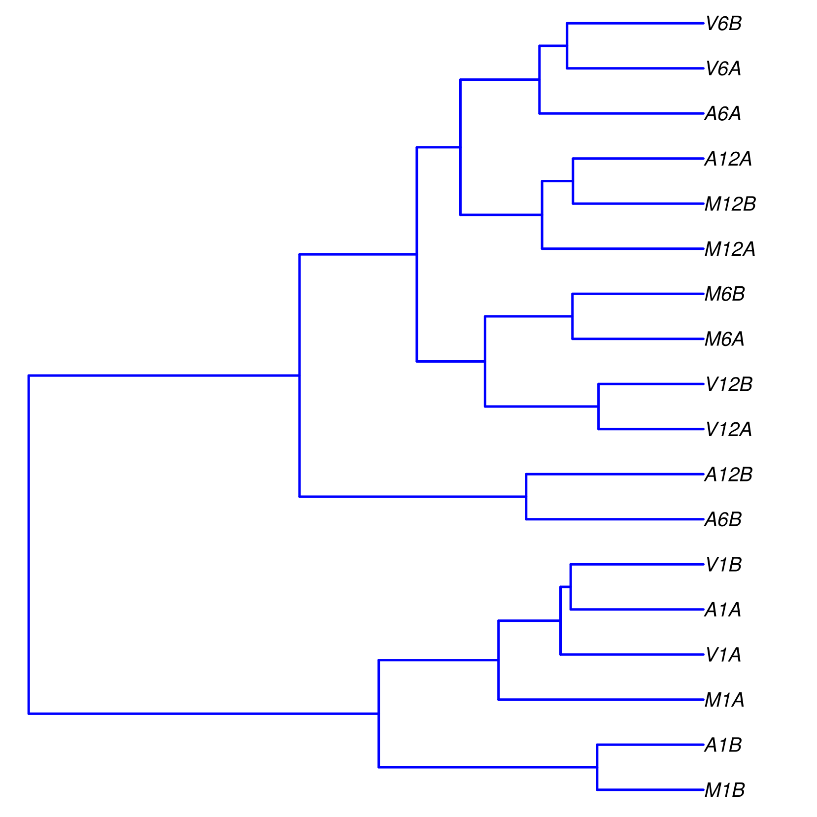
样本间的相关性分析

进行样本间的相关性分析。利用DESeq2包进行样本间相关性分析的过程。首先将计数数据导入，然后构建DESeq2数据集，并计算样本间的Spearman相关系数。最后，通过层次聚类和绘图，将相关性结果以聚类图的形式保存在PDF文件中。主要包括以下几个步骤：

导入所需的包：通过library函数导入了DESeq2和ape包，用于进行差异表达分析和绘制聚类图的操作。
读取计数数据：通过read.table函数将计数结果文件"results/countDFeByg.xls"读取为一个矩阵（countDF）。
构建DESeq2数据集：通过DESeqDataSetFromMatrix函数将计数数据（countDF）和条件数据（colData）构建为一个DESeq2数据集（dds），指定了条件设计。
计算相关系数：通过cor函数计算基于rlog转换后的表达值的Spearman相关系数。将rlog函数应用于DESeq2数据集（dds）的表达值，然后通过assay函数提取表达矩阵，并计算相关系数（d）。
层次聚类：通过hclust函数对距离矩阵（dist(1 - d)）进行层次聚类，生成聚类树对象（hc）。
绘制聚类图：通过pdf函数创建一个PDF文件（“results/sample_tree.pdf”），然后使用plot.phylo函数绘制聚类树（as.phylo(hc)），并设置图形的样式参数。
保存聚类图：通过dev.off函数关闭PDF文件，保存并生成聚类图文件。

## 4.2 Sample-wise correlation analysis
## The following computes the sample-wise Spearman correlation coefficients from the
## rlog transformed expression values generated with the DESeq2 package. After
## transformation to a distance matrix, hierarchical clustering is performed with the
## hclust function and the result is plotted as a dendrogram (also see file
## sample_tree.pdf).
library(DESeq2, quietly = TRUE)
library(ape, warn.conflicts = FALSE)
countDF <- as.matrix(read.table("./results/countDFeByg.xls"))
colData <- data.frame(row.names = targets.as.df(targets(args))$SampleName, 
                      condition = targets.as.df(targets(args))$Factor)
dds <- DESeqDataSetFromMatrix(countData = countDF, colData = colData, 
                              design = ~condition)
d <- cor(assay(rlog(dds)), method = "spearman")
hc <- hclust(dist(1 - d))
pdf("results/sample_tree.pdf")
plot.phylo(as.phylo(hc), type = "p", edge.col = "blue", edge.width = 2, 
           show.node.label = TRUE, no.margin = TRUE)
dev.off()

差异表达分析

运行edgeR

使用edgeR包进行差异表达分析的过程。通过读取计数数据和目标样本信息，定义比较组，运行edgeR分析，并将结果输出到文件中。另外，还使用biomaRt包获取基因描述信息，并将其添加到差异表达结果中。主要包括以下几个步骤：

导入所需的包：通过library函数导入了edgeR和biomaRt包，用于差异表达分析和获取基因描述信息的操作。
读取计数数据和目标样本信息：通过read.delim函数分别读取计数数据文件"results/countDFeByg.xls"和目标样本信息文件"targets.txt"。
定义比较组：通过readComp函数从目标样本信息中提取比较组信息，将其存储在变量cmp中。
运行edgeR：通过run_edgeR函数利用glm方法对计数数据进行差异表达分析。传入计数数据（countDF）、目标样本信息（targets）和比较组信息（cmp[[1]]），并指定independent = FALSE表示非独立比较。
添加基因描述信息：通过使用biomaRt包中的useMart和getBM函数，连接到植物数据库（plants_mart）并获取基因描述信息。将基因描述信息添加到差异表达结果（edgeDF）的数据框中。
输出结果：使用write.table函数将差异表达结果（edgeDF）写入到"./results/edgeRglm_allcomp.xls"文件中，以制表符分隔，不加引号，列名不写入文件。

## 5. Analysis of DEGs
#####################################################
## The analysis of differentially expressed genes (DEGs) is performed with the glm
## method of the edgeR package (Robinson, McCarthy, and Smyth 2010). The sample
## comparisons used by this analysis are defined in the header lines of the
## targets.txt file starting with <CMP>.

## 5.1 Run edgeR
library(edgeR)
countDF <- read.delim("results/countDFeByg.xls", row.names = 1, 
                      check.names = FALSE)
targets <- read.delim("targets.txt", comment = "#")
cmp <- readComp(file = "targets.txt", format = "matrix", delim = "-")
edgeDF <- run_edgeR(countDF = countDF, targets = targets, cmp = cmp[[1]], 
                    independent = FALSE, mdsplot = "")
## Add gene descriptions
library("biomaRt")
m <- useMart("plants_mart", dataset = "athaliana_eg_gene", host = "https://plants.ensembl.org")
desc <- getBM(attributes = c("tair_locus", "description"), mart = m)
desc <- desc[!duplicated(desc[, 1]), ]
descv <- as.character(desc[, 2])
names(descv) <- as.character(desc[, 1])
edgeDF <- data.frame(edgeDF, Desc = descv[rownames(edgeDF)], 
                     check.names = FALSE)
write.table(edgeDF, "./results/edgeRglm_allcomp.xls", quote = FALSE, 
            sep = "\t", col.names = NA)

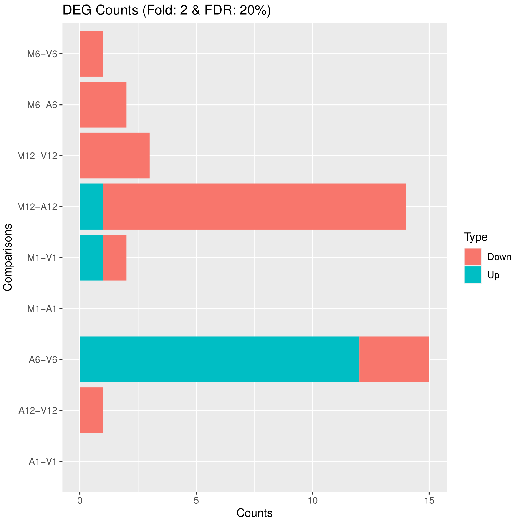
可视化差异表达结果

筛选和可视化差异表达结果，首先读取差异表达结果文件，然后根据设定的筛选条件进行筛选，并将筛选结果绘制成图形保存在PDF文件中。此外，还将筛选后的DEG统计结果输出到文件中。主要包括以下几个步骤：

读取差异表达结果：通过read.delim函数读取差异表达结果文件"results/edgeRglm_allcomp.xls"。
绘制DEG结果图：通过pdf函数创建一个PDF文件（“results/DEGcounts.pdf”），然后使用filterDEGs函数对差异表达结果进行筛选和绘图。筛选条件通过filter参数指定，其中包括折叠变化（Fold）和调整的p值（FDR）。绘图结果保存在PDF文件中。
输出DEG统计结果：使用write.table函数将DEG结果的摘要信息（DEG_list$Summary）写入到"./results/DEGcounts.xls"文件中，以制表符分隔，不加引号，不写入行名。

## 5.2 Plot DEG results
## Filter and plot DEG results for up and down regulated genes. The definition of up
## and down is given in the corresponding help file. To open it, type ?filterDEGs in
## the R console.
edgeDF <- read.delim("results/edgeRglm_allcomp.xls", row.names = 1, 
                     check.names = FALSE)
pdf("results/DEGcounts.pdf")
DEG_list <- filterDEGs(degDF = edgeDF, filter = c(Fold = 2, FDR = 20))
dev.off()
write.table(DEG_list$Summary, "./results/DEGcounts.xls", quote = FALSE, 
            sep = "\t", row.names = FALSE)

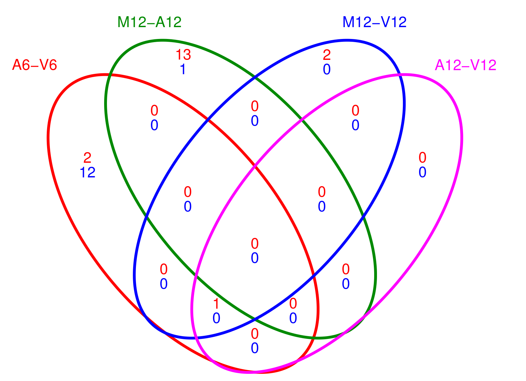
计算和绘制差异表达基因（DEG）集合的Venn图

利用overLapper和vennPlot函数计算和绘制差异表达基因集合的Venn图。首先计算上调和下调基因集合的Venn图交集，并将结果保存。然后根据设定绘制Venn图，并将图形保存到PDF文件中。主要包括以下几个步骤：

创建Venn图数据：通过overLapper函数计算DEG集合的Venn图交集。首先使用DEG_list$Up[6:9]作为输入，表示选取DEG结果中上调基因的第6至第9个集合，然后将结果保存在vennsetup变量中。接着，使用DEG_list$Down[6:9]作为输入，表示选取DEG结果中下调基因的第6至第9个集合，将结果保存在vennsetdown变量中。
绘制Venn图：通过pdf函数创建一个PDF文件（“results/vennplot.pdf”），然后使用vennPlot函数绘制Venn图。将需要绘制的Venn图数据传入list函数中，并通过mymain和mysub参数指定主标题和副标题为空字符串。此外，colmode参数设为2表示使用两种颜色（蓝色和红色）来区分上调和下调的基因集合。
结束绘图：通过dev.off函数结束图形设备，保存Venn图到PDF文件中。

## 5.3 Venn diagrams of DEG sets
## The overLapper function can compute Venn intersects for large numbers of sample
## sets (up to 20 or more) and plots 2-5 way Venn diagrams. A useful feature is the
## possibility to combine the counts from several Venn comparisons with the same
## number of sample sets in a single Venn diagram (here for 4 up and down DEG sets).
vennsetup <- overLapper(DEG_list$Up[6:9], type = "vennsets")
vennsetdown <- overLapper(DEG_list$Down[6:9], type = "vennsets")
pdf("results/vennplot.pdf")
vennPlot(list(vennsetup, vennsetdown), mymain = "", mysub = "", 
         colmode = 2, ccol = c("blue", "red"))
dev.off()

GO富集分析

准备工作

进行基因-基因本体（Gene Ontology, GO）富集分析的准备工作。首先选择并获取BioMart数据库，然后从数据库中获取基因到GO的映射关系，并对结果进行预处理。最后，创建基因到GO的CATdb对象用于后续的GO富集分析。主要包括以下几个步骤：

选择和获取BioMart数据库：通过使用listMarts函数列出可用的BioMart数据库，选择目标数据库。在这里，通过指定host参数为"https://plants.ensembl.org"来获取与植物相关的数据库。然后使用useMart函数选择目标数据库和数据集。
获取基因到GO映射：通过使用getBM函数从选择的BioMart数据库中获取基因到GO的映射关系。指定所需的属性（attributes）为"go_id"（GO标识符）、“tair_locus”（基因标识符）和"namespace_1003"（GO的命名空间）。将获取的结果保存在go变量中。
数据预处理：对获取的基因到GO映射进行预处理。首先，去除命名空间为空的条目。然后，将命名空间的值转换为缩写形式（"F"表示分子功能，"P"表示生物过程，"C"表示细胞组分）。最后，将结果保存在文件"GOannotationsBiomart_mod.txt"中。
创建基因到GO的CATdb对象：通过使用makeCATdb函数创建基因到GO的CATdb对象。指定文件路径、列号以及其他必要的参数。将创建的CATdb对象保存在文件"catdb.RData"中。

## 6. GO term enrichment analysis
#####################################################
## 6.1 Obtain gene-to-GO mappings
## The following shows how to obtain gene-to-GO mappings from biomaRt (here for
## A. thaliana) and how to organize them for the downstream GO term enrichment
## analysis. Alternatively, the gene-to-GO mappings can be obtained for many
## organisms from Bioconductor’s *.db genome annotation packages or GO
## annotation files provided by various genome databases. For each annotation this
## relatively slow preprocessing step needs to be performed only once. Subsequently,
## the preprocessed data can be loaded with the load function as shown in the next
## subsection.
library("biomaRt")
listMarts()  # To choose BioMart database
listMarts(host = "https://plants.ensembl.org")
m <- useMart("plants_mart", host = "https://plants.ensembl.org")
listDatasets(m)
m <- useMart("plants_mart", dataset = "athaliana_eg_gene", host = "https://plants.ensembl.org")
listAttributes(m)  # Choose data types you want to download
go <- getBM(attributes = c("go_id", "tair_locus", "namespace_1003"), 
            mart = m)
# If download fail, you can load the following Rdata.
#load("Lab_4 files/go.Rdata")
go <- go[go[, 3] != "", ]
go[, 3] <- as.character(go[, 3])
go[go[, 3] == "molecular_function", 3] <- "F"
go[go[, 3] == "biological_process", 3] <- "P"
go[go[, 3] == "cellular_component", 3] <- "C"
go[1:4, ]
# dir.create("./data/GO")
write.table(go, "data/GO/GOannotationsBiomart_mod.txt", quote = FALSE, 
            row.names = FALSE, col.names = FALSE, sep = "\t")
catdb <- makeCATdb(myfile = "data/GO/GOannotationsBiomart_mod.txt", 
                   lib = NULL, org = "", colno = c(1, 2, 3), idconv = NULL)
save(catdb, file = "data/GO/catdb.RData")

批量进行GO富集分析

这段代码主要用于进行批量的基因本体（Gene Ontology, GO）富集分析，首先根据DEG结果定义DEG集合，然后执行批量的GO富集分析和GO slim富集分析。最后，将结果保存在相应的变量中。具体步骤如下：

载入所需的包和数据：通过加载"biomaRt"包和预处理好的基因到GO的CATdb对象（从之前的代码段中加载）。同时，也加载了之前进行差异表达分析得到的DEG结果（DEG_list）。
定义DEG集合：根据DEG结果，将上调和下调基因分别命名为"名称_up_down"、"名称_up"和"名称_down"的命名空间。创建DEG集合（DEGlist）将这些命名空间组合起来，并移除长度为0的集合。
执行批量的GO富集分析：使用GOCluster_Report函数对DEG集合进行批量的GO富集分析。设置方法参数（method）为"all"，表示返回所有通过设定的p-value阈值（cutoff）的GO术语。指定id_type参数为"gene"，表示基因标识符类型。还可以设置其他参数，如聚类阈值（CLSZ）、GO分类（gocats）和记录指定的GO术语（recordSpecGO）。将结果保存在BatchResult变量中。
获取GO slim向量：通过使用"biomaRt"包获取特定生物体的GO slim向量。选择合适的BioMart数据库（“plants_mart”）和数据集（“athaliana_eg_gene”），然后使用getBM函数获取"goslim_goa_accession"属性并将结果转换为字符向量。
执行GO slim富集分析：使用GOCluster_Report函数对DEG集合进行GO slim富集分析。设置方法参数（method）为"slim"，表示仅返回在"goslimvec"向量中指定的GO术语。其他参数的设置与批量GO富集分析类似。将结果保存在BatchResultslim变量中。

## 6.2 Batch GO term enrichment analysis
## Apply the enrichment analysis to the DEG sets obtained the above differential
## expression analysis. Note, in the following example the FDR filter is set here to an
## unreasonably high value, simply because of the small size of the toy data set used ## in
## this vignette. Batch enrichment analysis of many gene sets is performed with the
## function. When method=all, it returns all GO terms passing the p-value cutoff
## specified under the cutoff arguments. When method=slim, it returns only the GO
## terms specified under the myslimv argument. The given example shows how a GO
## slim vector for a specific organism can be obtained from BioMart.
library("biomaRt")
load("data/GO/catdb.RData")
DEG_list <- filterDEGs(degDF = edgeDF, filter = c(Fold = 2, FDR = 50), 
                       plot = FALSE)
up_down <- DEG_list$UporDown
names(up_down) <- paste(names(up_down), "_up_down", sep = "")
up <- DEG_list$Up
names(up) <- paste(names(up), "_up", sep = "")
down <- DEG_list$Down
names(down) <- paste(names(down), "_down", sep = "")
DEGlist <- c(up_down, up, down)
DEGlist <- DEGlist[sapply(DEGlist, length) > 0]
BatchResult <- GOCluster_Report(catdb = catdb, setlist = DEGlist, 
                                method = "all", id_type = "gene", CLSZ = 2, cutoff = 0.9, 
                                gocats = c("MF", "BP", "CC"), recordSpecGO = NULL)
library("biomaRt")
m <- useMart("plants_mart", dataset = "athaliana_eg_gene", host = "https://plants.ensembl.org")
goslimvec <- as.character(getBM(attributes = c("goslim_goa_accession"), 
                                mart = m)[, 1])
BatchResultslim <- GOCluster_Report(catdb = catdb, setlist = DEGlist, 
                                    method = "slim", id_type = "gene", myslimv = goslimvec, CLSZ = 10, 
                                    cutoff = 0.01, gocats = c("MF", "BP", "CC"), recordSpecGO = NULL)

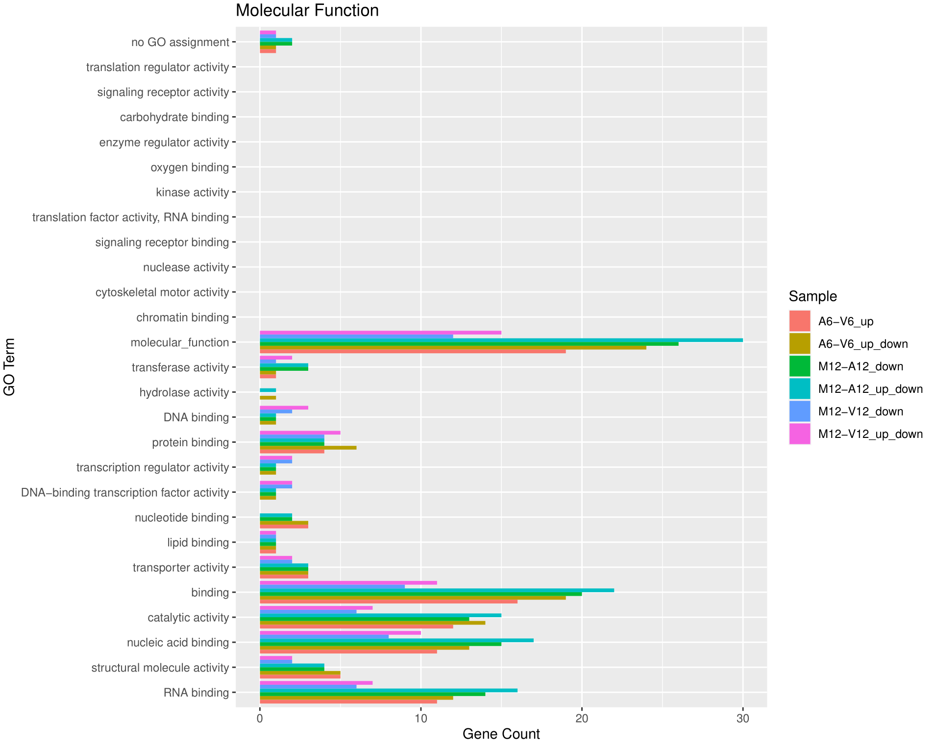
绘制批量GO富集分析的结果

使用goBarplot函数绘制批量GO富集分析结果的条形图。首先选择感兴趣的子集，然后分别绘制不同GO类别的条形图。具体步骤如下：

子集选择：首先从BatchResultslim数据框中选择与"M6-V6_up_down"匹配的行，将结果存储在gos变量中。然后将整个BatchResultslim数据框存储在gos变量中，以便后续绘制。
绘制MF（分子功能）类别的GO条形图：通过调用goBarplot函数绘制MF类别的GO条形图。将gos作为输入数据框，并设置gocat参数为"MF"。将结果保存为PDF文件。
绘制BP（生物过程）类别的GO条形图：通过再次调用goBarplot函数绘制BP类别的GO条形图。将gos作为输入数据框，并设置gocat参数为"BP"。
绘制CC（细胞组分）类别的GO条形图：通过再次调用goBarplot函数绘制CC类别的GO条形图。将gos作为输入数据框，并设置gocat参数为"CC"。

## 6.3 Plot batch GO term results
## The data.frame generated by GOCluster can be plotted with the goBarplot
## function. Because of the variable size of the sample sets, it may not always be
## desirable to show the results from different DEG sets in the same bar plot. Plotting
## single sample sets is achieved by subsetting the input data frame as shown in the
## first line of the following example.
gos <- BatchResultslim[grep("M6-V6_up_down", BatchResultslim$CLID), 
]
gos <- BatchResultslim
pdf("GOslimbarplotMF.pdf", height = 8, width = 10)
goBarplot(gos, gocat = "MF")
dev.off()
goBarplot(gos, gocat = "BP")
goBarplot(gos, gocat = "CC")

这里以分子功能为例。

层次聚类和热图绘制

使用pheatmap库进行层次聚类和热图绘制。首先提取感兴趣基因的表达矩阵子集，然后基于Pearson相关系数计算距离并进行层次聚类，最后绘制热图以可视化聚类结果。具体步骤如下：

导入必要的库：通过加载pheatmap库，准备进行层次聚类和热图分析。
提取差异表达基因（DEGs）的表达矩阵：从上述差异表达分析中确定的DEGs中提取基因的rlog转换后的表达矩阵。这里使用了DEG_list[[1]]作为DEGs的标识，通过将其转换为字符向量并去除重复项，得到基因的唯一标识符。
提取感兴趣基因的表达值：从rlog转换后的表达矩阵中，提取与感兴趣基因的唯一标识符相对应的行，得到一个子集矩阵y。
绘制热图：通过调用pheatmap函数绘制热图。设置scale参数为"row"，对行进行标准化；设置clustering_distance_rows参数和clustering_distance_cols参数为"correlation"，使用基于Pearson相关系数的距离度量进行行和列的层次聚类。将结果保存为PDF文件。

## 7. Clustering and heat maps
#####################################################
## The following example performs hierarchical clustering on the rlog transformed
## expression matrix subsetted by the DEGs identified in the above differential
## expression analysis. It uses a Pearson correlation-based distance measure and
## complete linkage for cluster joining.
library(pheatmap)
geneids <- unique(as.character(unlist(DEG_list[[1]])))
y <- assay(rlog(dds))[geneids, ]
pdf("heatmap1.pdf")
pheatmap(y, scale = "row", clustering_distance_rows = "correlation", 
         clustering_distance_cols = "correlation")
dev.off()

RDEKA[3V5VGK4]DURRNWX%F