第一部分 认识CNN

一、quickly start

所见即所得，先看一下CNN在MNIST上的运行Demo

from keras import layers
from keras import models

model = models.Sequential()
# 定义一个卷积输入层，卷积核是3*3，共32个，输入是(28, 28, 1)，输出是(26, 26, 32)
model.add(layers.Conv2D(32, (3, 3), activation='relu', input_shape=(28, 28, 1)))
# 定义一个2*2的池化层
model.add(layers.MaxPooling2D((2, 2)))
model.add(layers.Conv2D(64, (3, 3), activation='relu'))
model.add(layers.MaxPooling2D((2, 2)))
model.add(layers.Conv2D(64, (3, 3), activation='relu'))
# 将所有的输出展平
model.add(layers.Flatten())
# 定义一个全连接层，有64个神经元
model.add(layers.Dense(64, activation='relu'))
# 多分类问题，将输出在每个分类上的概率
model.add(layers.Dense(10, activation='softmax'))
model.summary()

打印网络结构

_________________________________________________________________
Model: "sequential_1"
_________________________________________________________________
Layer (type)                 Output Shape              Param #   
_________________________________________________________________
conv2d_1 (Conv2D)            (None, 26, 26, 32)        320       
_________________________________________________________________
max_pooling2d_1 (MaxPooling2 (None, 13, 13, 32)        0         
_________________________________________________________________
conv2d_2 (Conv2D)            (None, 11, 11, 64)        18496     
_________________________________________________________________
max_pooling2d_2 (MaxPooling2 (None, 5, 5, 64)          0         
_________________________________________________________________
conv2d_3 (Conv2D)            (None, 3, 3, 64)          36928     
_________________________________________________________________
flatten_1 (Flatten)          (None, 576)               0         
_________________________________________________________________
dense_1 (Dense)              (None, 64)                36928     
_________________________________________________________________
dense_2 (Dense)              (None, 10)                650       
_________________________________________________________________
Total params: 93,322
Trainable params: 93,322
Non-trainable params: 0
_________________________________________________________________

加载数据开始训练

from keras.datasets import mnist
from keras.utils import to_categorical

(train_images, train_labels), (test_images, test_labels) = mnist.load_data()

train_images = train_images.reshape((60000, 28, 28, 1))
train_images = train_images.astype('float32') / 255

test_images = test_images.reshape((10000, 28, 28, 1))
test_images = test_images.astype('float32') / 255

train_labels = to_categorical(train_labels)
test_labels = to_categorical(test_labels)
print('train data:', train_images.shape, train_labels.shape)
print('test data:', test_images.shape, test_labels.shape)

# 训练数据准确的已经明显优于全连接网络
model.compile(optimizer='rmsprop',
              loss='categorical_crossentropy',
              metrics=['accuracy'])
model.fit(train_images, train_labels, epochs=5, batch_size=64)
test_loss, test_acc = model.evaluate(test_images, test_labels)
print(test_loss, test_acc)

train data: (60000, 28, 28, 1) (60000, 10)
test data: (10000, 28, 28, 1) (10000, 10)
0.025266158195689788
0.9919000267982483

二、卷积网络介绍

全连接层与卷积层根本的区别在于，全连接层从输入特征空间中学到的是全局模式，而卷积层学到的是局部模式

• 卷积神经网络具有平移不变性，一个地方学到的识别能力可以用到其他的任何地方
• 卷积神经网络可以学到模式的空间层次结构

# CNN在Keras上的API
tf.keras.layers.Conv2D(
    filters, # 卷积核的个数
    kernel_size, # 卷积核的大小，常用的是（3，3）
    strides=(1, 1), # 核移动步幅
    padding='valid', # 是否需要边界填充
    data_format=None,
    dilation_rate=(1, 1), 
    activation=None, # 激活函数
    use_bias=True,
    kernel_initializer='glorot_uniform',
    bias_initializer='zeros',
    kernel_regularizer=None, 
    bias_regularizer=None, 
    activity_regularizer=None,
    kernel_constraint=None, 
    bias_constraint=None, 
    **kwargs
)

2.1 卷积核运算

卷积计算类似于点积，一个矩阵(3, 3, 2)卷积(3, 3, 2)的结果是(1)
如上图所示：
输入为 (5, 5, 2) （高， 宽， 深度）
卷积核为 (3, 3, 2)
一个卷积核的输出为 (3, 3, 1)
三个卷积核的输出为 (3, 3, 3)
图中输出深度(1, 1, 3)表示的是三个卷积核在一个位置上的输出

2.2 边界填充Padding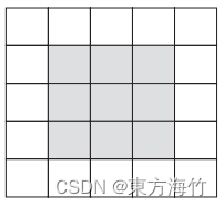

边界填充的目的是为了充分发掘边界的信息，确保每个点都成为过核心，所以
对于(3, 3)的卷积核，我们往左右同时增加一列；
对于(5, 5)的卷积核，我们左右同时增加两列。
参数padding='same’表示需要边界填充

2.3 卷积步幅strides

步幅很好理解，就是卷积核计算完后需要往下一格挪动几个位置

2.4 最大池化层MaxPooling

最大池化层通常使用2*2的窗口，步幅为2进行特征下采样
作用有二：
1、减少需要处理的特征图的元素个数
2、增加卷积层的观察窗口（即窗口覆盖原始输入的比例越来越大）
一个张量输入(28, 28, 32)，经过(2, 2)的MaxPooling处理，输出张量(14, 14, 32)，其过程直观的可以理解为取相邻(2, 2)矩阵里面的最大值。当然也有其他的处理方法，比如取平均值。

第二部分：CNN在Keras上的实践

一、做好基础数据准备

实践案例：猫狗分类
数据下载：https://www.kaggle.com/c/dogs-vs-cats/data
源数据： 2000 张猫的图像 + 2000 张狗的图像
数据划分： 2000 张训练，1000 张验证，1000张测试

• 数据准备，从下载好的数据中清洗出源数据
  目录结构：
  cat-dog-small
  ├─test
    │ ├─cats 500张
    │ └─dogs 500张
  ├─train
    │ ├─cats 1000张
    │ └─dogs 1000张
  └─validation
  ├─cats 500张
  └─dogs 500张

import os, shutil
# The path to the directory where the original
# dataset was uncompressed
original_dataset_dir = 'D://Kaggle//cat-dog//train'

# The directory where we will
# store our smaller dataset
base_dir = 'D://Kaggle//cat-dog-small'
os.mkdir(base_dir)

# Directories for our training splits
train_dir = os.path.join(base_dir, 'train')
os.mkdir(train_dir)
train_cats_dir = os.path.join(train_dir, 'cats')
os.mkdir(train_cats_dir)
train_dogs_dir = os.path.join(train_dir, 'dogs')
os.mkdir(train_dogs_dir)

# Directories for our validation splits
validation_dir = os.path.join(base_dir, 'validation')
os.mkdir(validation_dir)
validation_cats_dir = os.path.join(validation_dir, 'cats')
os.mkdir(validation_cats_dir)
validation_dogs_dir = os.path.join(validation_dir, 'dogs')
os.mkdir(validation_dogs_dir)

# Directories for our test splits
test_dir = os.path.join(base_dir, 'test')
os.mkdir(test_dir)
test_cats_dir = os.path.join(test_dir, 'cats')
os.mkdir(test_cats_dir)
test_dogs_dir = os.path.join(test_dir, 'dogs')
os.mkdir(test_dogs_dir)

# Copy first 1000 cat images to train_cats_dir
fnames = ['cat.{}.jpg'.format(i) for i in range(1000)]
for fname in fnames:
    src = os.path.join(original_dataset_dir, fname)
    dst = os.path.join(train_cats_dir, fname)
    shutil.copyfile(src, dst)

# Copy next 500 cat images to validation_cats_dir
fnames = ['cat.{}.jpg'.format(i) for i in range(1000, 1500)]
for fname in fnames:
    src = os.path.join(original_dataset_dir, fname)
    dst = os.path.join(validation_cats_dir, fname)
    shutil.copyfile(src, dst)
    
# Copy next 500 cat images to test_cats_dir
fnames = ['cat.{}.jpg'.format(i) for i in range(1500, 2000)]
for fname in fnames:
    src = os.path.join(original_dataset_dir, fname)
    dst = os.path.join(test_cats_dir, fname)
    shutil.copyfile(src, dst)
    
# Copy first 1000 dog images to train_dogs_dir
fnames = ['dog.{}.jpg'.format(i) for i in range(1000)]
for fname in fnames:
    src = os.path.join(original_dataset_dir, fname)
    dst = os.path.join(train_dogs_dir, fname)
    shutil.copyfile(src, dst)
    
# Copy next 500 dog images to validation_dogs_dir
fnames = ['dog.{}.jpg'.format(i) for i in range(1000, 1500)]
for fname in fnames:
    src = os.path.join(original_dataset_dir, fname)
    dst = os.path.join(validation_dogs_dir, fname)
    shutil.copyfile(src, dst)
    
# Copy next 500 dog images to test_dogs_dir
fnames = ['dog.{}.jpg'.format(i) for i in range(1500, 2000)]
for fname in fnames:
    src = os.path.join(original_dataset_dir, fname)
    dst = os.path.join(test_dogs_dir, fname)
    shutil.copyfile(src, dst)

• 数据处理，一切都仰仗于ImageDataGenerator
  按批次的从指定目录中获得图片，并解码、归一化
  真的很方便、省心、稳

from keras.preprocessing.image import ImageDataGenerator

# All images will be rescaled by 1./255
train_datagen = ImageDataGenerator(rescale=1./255)
validation_datagen = ImageDataGenerator(rescale=1./255)
test_datagen = ImageDataGenerator(rescale=1./255)

# 分批次的将数据按目录读取出来，ImageDataGenerator会一直取图片，直到break
train_generator = train_datagen.flow_from_directory(
        # This is the target directory
        train_dir,
        # All images will be resized to 150x150
        target_size=(150, 150),
        batch_size=20,
        # Since we use binary_crossentropy loss, we need binary labels
        class_mode='binary')

validation_generator = validation_datagen.flow_from_directory(
        validation_dir,
        target_size=(150, 150),
        batch_size=20,
        class_mode='binary')

test_generator = test_datagen.flow_from_directory(
        test_dir,
        target_size=(150, 150),
        batch_size=20,
        class_mode='binary')

Found 2000 images belonging to 2 classes.
Found 1000 images belonging to 2 classes.
Found 1000 images belonging to 2 classes.

二、模型迭代

实践流程：
训练一个无任何优化的基准版本（acc 0.700）
----> 加入了数据增强的版本（acc 0.810）
----> 用预训练好的网络（acc 0.893）
----> 数据增强+预训练好的网络（acc 0.904）
----> 微调预训练的网络（acc 0.924）
----> 数据增强+微调预训练的网络（acc ）
----> 待续（acc ）
简而言之，越来越耗时，越来越准

2.1 基准网络，全凭灵感

我们搭建起一个四卷积层、四MaxPooling、一展开层、一全连接层、一输出层的基准网络

from keras import layers
from keras import models

model1 = models.Sequential()
model1.add(layers.Conv2D(32, (3, 3), activation='relu', input_shape=(150, 150, 3)))
model1.add(layers.MaxPooling2D((2, 2)))
model1.add(layers.Conv2D(64, (3, 3), activation='relu'))
model1.add(layers.MaxPooling2D((2, 2)))
model1.add(layers.Conv2D(128, (3, 3), activation='relu'))
model1.add(layers.MaxPooling2D((2, 2)))
model1.add(layers.Conv2D(128, (3, 3), activation='relu'))
model1.add(layers.MaxPooling2D((2, 2)))
model1.add(layers.Flatten())
model1.add(layers.Dense(512, activation='relu'))
model1.add(layers.Dense(1, activation='sigmoid'))
model1.summary()

Model: "sequential_3"
_________________________________________________________________
Layer (type)                 Output Shape              Param #   
=================================================================
conv2d_8 (Conv2D)            (None, 148, 148, 32)      896       
_________________________________________________________________
max_pooling2d_7 (MaxPooling2 (None, 74, 74, 32)        0         
_________________________________________________________________
conv2d_9 (Conv2D)            (None, 72, 72, 64)        18496     
_________________________________________________________________
max_pooling2d_8 (MaxPooling2 (None, 36, 36, 64)        0         
_________________________________________________________________
conv2d_10 (Conv2D)           (None, 34, 34, 128)       73856     
_________________________________________________________________
max_pooling2d_9 (MaxPooling2 (None, 17, 17, 128)       0         
_________________________________________________________________
conv2d_11 (Conv2D)           (None, 15, 15, 128)       147584    
_________________________________________________________________
max_pooling2d_10 (MaxPooling (None, 7, 7, 128)         0         
_________________________________________________________________
flatten_3 (Flatten)          (None, 6272)              0         
_________________________________________________________________
dense_5 (Dense)              (None, 512)               3211776   
_________________________________________________________________
dense_6 (Dense)              (None, 1)                 513       
=================================================================
Total params: 3,453,121
Trainable params: 3,453,121
Non-trainable params: 0
_________________________________________________________________

仔细介绍一下param参数的计算规则

• 全连接网络
  total_params = (input_data_channels + 1) * number_of_filters
  参数的总量等于一个神经元的参数量（W,b）乘上神经元个数

dense	filters	input_shape	output_shape
dense_5	512	(6272)	(None, 512)
params = (6272 + 1) * 522 = 3211776
dense_6	1	(512)	(None, 1)
params = (512 + 1) * 1 = 513

• 卷积网络
  total_params = (filter_height * filter_width * input_image_channels + 1) * number_of_filters
  参数的总量等于一个卷积核的参数量（W,b）乘上卷积核的个数

Conv2D	filters	kernel_size	input_shape	output_shape
conv2d_8	32	(3, 3)	(150, 150, 3)	(None, 148, 148, 32)
params = (3 * 3 * 3 + 1) * 32 = 896
conv2d_9	64	(3, 3)	(74, 74, 32)	(None, 72, 72, 64)
params = (3 * 3 * 32 + 1) * 64 = 18496
conv2d_10	128	(3, 3)	(36, 36, 64)	(None, 34, 34, 128)
params = (3 * 3 * 64 + 1) * 128 = 73856
conv2d_11	128	(3, 3)	(17, 17, 128)	(None, 15, 15, 128)
params = (3 * 3 * 128 + 1) * 128 = 147584

from keras import optimizers

model1.compile(loss='binary_crossentropy',
              optimizer=optimizers.RMSprop(lr=1e-4),
              metrics=['acc'])
history1 = model1.fit_generator(
      train_generator, # 训练数据生成器
      steps_per_epoch=100, # 每一个迭代需要读取100次生成器的数据
      epochs=30, # 迭代次数
      validation_data=validation_generator, # 验证数据生成器
      validation_steps=50) # 需要读取50次才能加载全部的验证集数据
      
# loss的波动幅度有点大
print(model1.metrics_names)
print(model1.evaluate_generator(test_generator, steps=50))

输出：
[‘loss’, ‘acc’]
[1.3509974479675293, 0.7329999804496765]
73%的准确率有点低，加油。

2.2 基准调优，数据增强

通过对ImageDataGenerator实例读取的图像执行多次随机变换不断的丰富训练样本

# 将 train_datagen = ImageDataGenerator(rescale=1./255)
# 修改为 
train_augmented_datagen = ImageDataGenerator(
    rescale=1./255,
    rotation_range=40, # 随机旋转的角度范围
    width_shift_range=0.2, # 在水平方向上平移的范围
    height_shift_range=0.2, # 在垂直方向上平移的范围
    shear_range=0.2, # 随机错切变换的角度
    zoom_range=0.2, # 随机缩放的范围
    horizontal_flip=True,)# 随机将一半图像水平翻转

# Note that the validation data should not be augmented!
train_augmented_generator = train_augmented_datagen.flow_from_directory(
        train_dir,
        target_size=(150, 150),
        batch_size=32,
        class_mode='binary')

介绍一下flow_from_directory函数的图像增强处理逻辑

先看flow_from_directory伪代码

xm,y=getDataIndex()#获取所有文件夹中所有图片索引，以及文件夹名也即标签

if shuffle==True:
    shuffle(xm,y)#打乱图片索引及其标签
while(True):
    for i in range(0,len(x),batch_size):
        xm_batch=xm[i:i+batch_size]#文件索引
        y_batch=y[i:i+batch_size]
        x_batch=getImg(xm_batch)#根据文件索引，获取图像数据
        ImagePro(x_batch)#数据增强
        #保存提升后的图片
        #saveToFile()
        yield (x_batch,y_batch)

顺序|乱序的将所有图片按张遍历、随机，然后重新开始遍历、随机，只要break不在，咱就不能停止造图片

# 重新训练一个模型
model2 = models.Sequential()
model2.add(layers.Conv2D(32, (3, 3), activation='relu', input_shape=(150, 150, 3)))
model2.add(layers.MaxPooling2D((2, 2)))
model2.add(layers.Conv2D(64, (3, 3), activation='relu'))
model2.add(layers.MaxPooling2D((2, 2)))
model2.add(layers.Conv2D(128, (3, 3), activation='relu'))
model2.add(layers.MaxPooling2D((2, 2)))
model2.add(layers.Conv2D(128, (3, 3), activation='relu'))
model2.add(layers.MaxPooling2D((2, 2)))
model2.add(layers.Flatten())
model2.add(layers.Dropout(0.5)) # 新加了dropout层
model2.add(layers.Dense(512, activation='relu'))
model2.add(layers.Dense(1, activation='sigmoid'))

model2.compile(loss='binary_crossentropy',
              optimizer=optimizers.RMSprop(lr=1e-4),
              metrics=['acc'])

history2 = model2.fit_generator(
      train_augmented_generator,
      steps_per_epoch=100, # 每一批次读取100轮数据，总共是3200张图片
      epochs=100,
      validation_data=validation_generator,
      validation_steps=50)

运行时间大幅度提升，之前每轮是40秒+，现在每轮是60秒+，acc也有所提升，也还需提升
[‘loss’, ‘acc’]
[0.3123816251754761, 0.8121827244758606]

2.3 VGG16，站在前人的肩上

利用卷积神经网络的可移植性，我们可以使用已经在大型数据集上训练号的网络，常见的有VGG、ResNet、Inception、Inception-ResNet，本篇主要是VGG16。
首先是下载VGG16网络

from keras.applications import VGG16

conv_base = VGG16(weights='imagenet', # 指定模型初始化的权重检查点
                  include_top=False, # 模型最后是否包含密集连接分类器，默认有1000个类别
                  input_shape=(150, 150, 3))
conv_base.summary()

输出网络结构

Model: "vgg16"
_________________________________________________________________
Layer (type)                 Output Shape              Param #   
=================================================================
input_2 (InputLayer)         (None, 150, 150, 3)       0         
_________________________________________________________________
block1_conv1 (Conv2D)        (None, 150, 150, 64)      1792      
_________________________________________________________________
block1_conv2 (Conv2D)        (None, 150, 150, 64)      36928     
_________________________________________________________________
block1_pool (MaxPooling2D)   (None, 75, 75, 64)        0         
_________________________________________________________________
block2_conv1 (Conv2D)        (None, 75, 75, 128)       73856     
_________________________________________________________________
block2_conv2 (Conv2D)        (None, 75, 75, 128)       147584    
_________________________________________________________________
block2_pool (MaxPooling2D)   (None, 37, 37, 128)       0         
_________________________________________________________________
block3_conv1 (Conv2D)        (None, 37, 37, 256)       295168    
_________________________________________________________________
block3_conv2 (Conv2D)        (None, 37, 37, 256)       590080    
_________________________________________________________________
block3_conv3 (Conv2D)        (None, 37, 37, 256)       590080    
_________________________________________________________________
block3_pool (MaxPooling2D)   (None, 18, 18, 256)       0         
_________________________________________________________________
block4_conv1 (Conv2D)        (None, 18, 18, 512)       1180160   
_________________________________________________________________
block4_conv2 (Conv2D)        (None, 18, 18, 512)       2359808   
_________________________________________________________________
block4_conv3 (Conv2D)        (None, 18, 18, 512)       2359808   
_________________________________________________________________
block4_pool (MaxPooling2D)   (None, 9, 9, 512)         0         
_________________________________________________________________
block5_conv1 (Conv2D)        (None, 9, 9, 512)         2359808   
_________________________________________________________________
block5_conv2 (Conv2D)        (None, 9, 9, 512)         2359808   
_________________________________________________________________
block5_conv3 (Conv2D)        (None, 9, 9, 512)         2359808   
_________________________________________________________________
block5_pool (MaxPooling2D)   (None, 4, 4, 512)         0         
=================================================================
Total params: 14,714,688
Trainable params: 14,714,688
Non-trainable params: 0
_________________________________________________________________

先来一个基础版本的——锁定卷积基
完全冻结所有的网络参数，只使用卷积基的输出训练新分类器

# 将（原始数据，label）转换为VGG16的（卷积基输出，label）
def extract_features(directory, sample_count):
    features = np.zeros(shape=(sample_count, 4, 4, 512)) # 卷积基最后一层的输出为(4， 4， 512)
    labels = np.zeros(shape=(sample_count))
    generator = datagen.flow_from_directory(
        directory,
        target_size=(150, 150),
        batch_size=batch_size,
        class_mode='binary')
    i = 0
    for inputs_batch, labels_batch in generator:
        features_batch = conv_base.predict(inputs_batch) # 直接以VGG16的输出作为训练分类器的features
        features[i * batch_size : (i + 1) * batch_size] = features_batch
        labels[i * batch_size : (i + 1) * batch_size] = labels_batch
        i += 1
        if i * batch_size >= sample_count:
            # Note that since generators yield data indefinitely in a loop,
            # we must `break` after every image has been seen once.
            break
    return features, labels

接下来只需要按照之前之前的步骤训练一个分类器即可，快得很

from keras import models
from keras import layers
from keras import optimizers

model3 = models.Sequential()
model3.add(layers.Dense(256, activation='relu', input_dim=4 * 4 * 512))
model3.add(layers.Dropout(0.5))
model3.add(layers.Dense(1, activation='sigmoid'))

model3.compile(optimizer=optimizers.RMSprop(lr=2e-5),
              loss='binary_crossentropy',
              metrics=['acc'])

history3 = model3.fit(train_features, train_labels,
                    epochs=30,
                    batch_size=20,
                    validation_data=(validation_features, validation_labels))

[‘loss’, ‘acc’]
[0.25353643798828124, 0.8930000066757202]
准确率已经到89%了，稳步提升中，

2.4 VGG16+数据增强，真强，也真慢

很自然，我们不满足于89%，我们自然会将数据加强融入其中，简单一点，直接将VGG16作为最终网络的一部分

from keras import models
from keras import layers

model4 = models.Sequential()
model4.add(conv_base)
model4.add(layers.Flatten())
model4.add(layers.Dense(256, activation='relu'))
model4.add(layers.Dense(1, activation='sigmoid'))
model4.summary()

输出网络结构

Model: "sequential_6"
_________________________________________________________________
Layer (type)                 Output Shape              Param #   
=================================================================
vgg16 (Model)                (None, 4, 4, 512)         14714688  
_________________________________________________________________
flatten_5 (Flatten)          (None, 8192)              0         
_________________________________________________________________
dense_11 (Dense)             (None, 256)               2097408   
_________________________________________________________________
dense_12 (Dense)             (None, 1)                 257       
=================================================================
Total params: 16,812,353
Trainable params: 16,812,353
Non-trainable params: 0 

继续感受一下1,681万参数带来的震撼
编译网络之前，我们需要固定卷积基

print('This is the number of trainable weights '
      'before freezing the conv base:', len(model4.trainable_weights))
      
conv_base.trainable = False

print('This is the number of trainable weights '
      'before freezing the conv base:', len(model4.trainable_weights))

输出

This is the number of trainable weights before freezing the conv base: 30
This is the number of trainable weights before freezing the conv base: 4

• 冻结之前
  VGG16一共19层，5个block，去掉1个输出层，5个MaxPolling层，剩下13层，再加上两个全连接层，总共15层，每层两个可训练权重（主权重W和偏置权重b），trainable_weights=(13+2)*2=30
• 冻结之后
  只有dense_11、dense_12两个全连接层可以训练，trainable_weights=2*2=4

准备编译

model4.compile(loss='binary_crossentropy',
              optimizer=optimizers.RMSprop(lr=2e-5),
              metrics=['acc'])

history4 = model4.fit_generator(
      train_augmented_generator,
      steps_per_epoch=100, # 3200个输入图片，增强
      epochs=60,
      validation_data=validation_generator,
      validation_steps=50,
      verbose=2)

model4.save('D://tmp//models//cats_and_dogs_small_4.h5')
print(model4.metrics_names)
print(model4.evaluate_generator(test_generator, steps=50))

[‘loss’, ‘acc’]
[0.23142974078655243, 0.9049999713897705]
之前一轮耗时60秒+，现在也就200秒+吧…好歹是acc上了90%
继续前行

2.5 锁定部分卷积基，微调模型

我们都知道越是靠近顶端（近输出层）的卷积层识别的内容越收敛于具体问题，一般优化思路就是组件的从顶端开始逐渐释放固定参数，适应当前问题

from keras import models
from keras import layers

model5 = models.Sequential()
model5.add(conv_base)
model5.add(layers.Flatten())
model5.add(layers.Dense(256, activation='relu'))
model5.add(layers.Dense(1, activation='sigmoid'))
model5.summary()

将block5整个解放

# 分别是block5_conv1、block5_conv2、block5_conv3、block5_pool 
conv_base.trainable = True

set_trainable = False
for layer in conv_base.layers:
    if layer.name == 'block5_conv1':
        set_trainable = True
    if set_trainable:
        layer.trainable = True
    else:
        layer.trainable = False

切记，一定是在编译之前操作

model5.compile(loss='binary_crossentropy',
              optimizer=optimizers.RMSprop(lr=1e-5),
              metrics=['acc'])

history5 = model5.fit_generator(
      train_generator,
      steps_per_epoch=100,
      epochs=100,
      validation_data=validation_generator,
      validation_steps=50)

print(model5.metrics_names)
print(model5.evaluate_generator(test_generator, steps=50))

[‘loss’, ‘acc’]
[1.8584696054458618, 0.9240000247955322]
训练集acc稳定在1，92%的acc还不够，训练集需要增强，模型参数也需要持续优化。
长路漫漫待你闯。

第三部分：CNN可视化

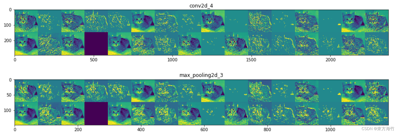
一、可视化网络中每一层的激活效果

可视化一下基准网络的每个卷积核激活效果

from keras.models import load_model
# 加载回来
model = load_model('D://tmp//models//cats_and_dogs_small_1.h5')
model.summary()  # As a reminder.

回忆下网络结构

Model: "sequential_2"
_________________________________________________________________
Layer (type)                 Output Shape              Param #   
=================================================================
conv2d_4 (Conv2D)            (None, 148, 148, 32)      896       
_________________________________________________________________
max_pooling2d_3 (MaxPooling2 (None, 74, 74, 32)        0         
_________________________________________________________________
conv2d_5 (Conv2D)            (None, 72, 72, 64)        18496     
_________________________________________________________________
max_pooling2d_4 (MaxPooling2 (None, 36, 36, 64)        0         
_________________________________________________________________
conv2d_6 (Conv2D)            (None, 34, 34, 128)       73856     
_________________________________________________________________
max_pooling2d_5 (MaxPooling2 (None, 17, 17, 128)       0         
_________________________________________________________________
conv2d_7 (Conv2D)            (None, 15, 15, 128)       147584    
_________________________________________________________________
max_pooling2d_6 (MaxPooling2 (None, 7, 7, 128)         0         
_________________________________________________________________
flatten_2 (Flatten)          (None, 6272)              0         
_________________________________________________________________
dense_3 (Dense)              (None, 512)               3211776   
_________________________________________________________________
dense_4 (Dense)              (None, 1)                 513       
=================================================================
Total params: 3,453,121
Trainable params: 3,453,121
Non-trainable params: 0
_________________________________________________________________

加载一张cat的照片，顺便体会一下ImageDataGenerator的便利

# 加载一张测试图片
img_path = 'D://Kaggle//cat-dog-small//test/cats//cat.1574.jpg'

# We preprocess the image into a 4D tensor
from keras.preprocessing import image
import numpy as np

img = image.load_img(img_path, target_size=(150, 150))
img_tensor = image.img_to_array(img)
img_tensor = np.expand_dims(img_tensor, axis=0)
# Remember that the model was trained on inputs
# that were preprocessed in the following way:
img_tensor /= 255.

# Its shape is (1, 150, 150, 3)
print(img_tensor.shape)

import matplotlib.pyplot as plt

plt.imshow(img_tensor[0])
plt.show()

先从model里将layer的output获得
再通过input、output构建一个model
predict可以获得所有的卷积核处理图片后的channel_image

from keras import models

# Extracts the outputs of the top 8 layers:
layer_outputs = [layer.output for layer in model.layers[:8]]
# Creates a model that will return these outputs, given the model input:
activation_model = models.Model(inputs=model.input, outputs=layer_outputs)

# This will return a list of 5 Numpy arrays:
# one array per layer activation
activations = activation_model.predict(img_tensor)

分层的将channel_image打印出来

import keras

# These are the names of the layers, so can have them as part of our plot
layer_names = []
for layer in model.layers[:8]:
    layer_names.append(layer.name)

# 一行16张图片
images_per_row = 16

# Now let's display our feature maps
for layer_name, layer_activation in zip(layer_names, activations):
    # 每一层都会有n_features张图片
    # This is the number of features in the feature map
    n_features = layer_activation.shape[-1]

    # The feature map has shape (1, size, size, n_features)
    size = layer_activation.shape[1]

    # We will tile the activation channels in this matrix
    n_cols = n_features // images_per_row 
    display_grid = np.zeros((size * n_cols, images_per_row * size))

    # We'll tile each filter into this big horizontal grid
    for col in range(n_cols):
        for row in range(images_per_row):
            channel_image = layer_activation[0,
                                             :, :,
                                             col * images_per_row + row]
            # 尤为关键
            # Post-process the feature to make it visually palatable
            channel_image -= channel_image.mean()
            channel_image /= channel_image.std()
            channel_image *= 64
            channel_image += 128
            channel_image = np.clip(channel_image, 0, 255).astype('uint8')
            display_grid[col * size : (col + 1) * size,
                         row * size : (row + 1) * size] = channel_image

    # Display the grid
    scale = 1. / size
    plt.figure(figsize=(scale * display_grid.shape[1],
                        scale * display_grid.shape[0]))
    plt.title(layer_name)
    plt.grid(False)
    plt.imshow(display_grid, aspect='auto', cmap='viridis')
    
plt.show()

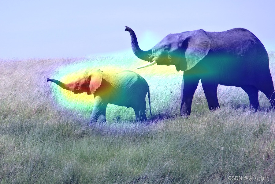
二、可视化激活的热力图

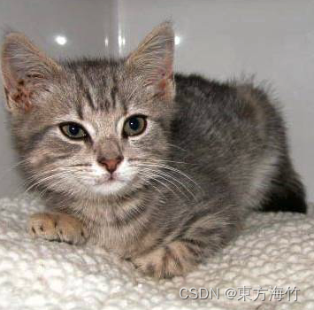
通过热力图我们可以直观的看到CNN是根据原始图像的哪一部分进行分类的
画热力图的方法是，
使用“每个通道对类别的重要程度”对“输入图像对不同通道的激活强度”的空间图进行加权，从而得到了“输入图像对类别的激活强度”的空间图
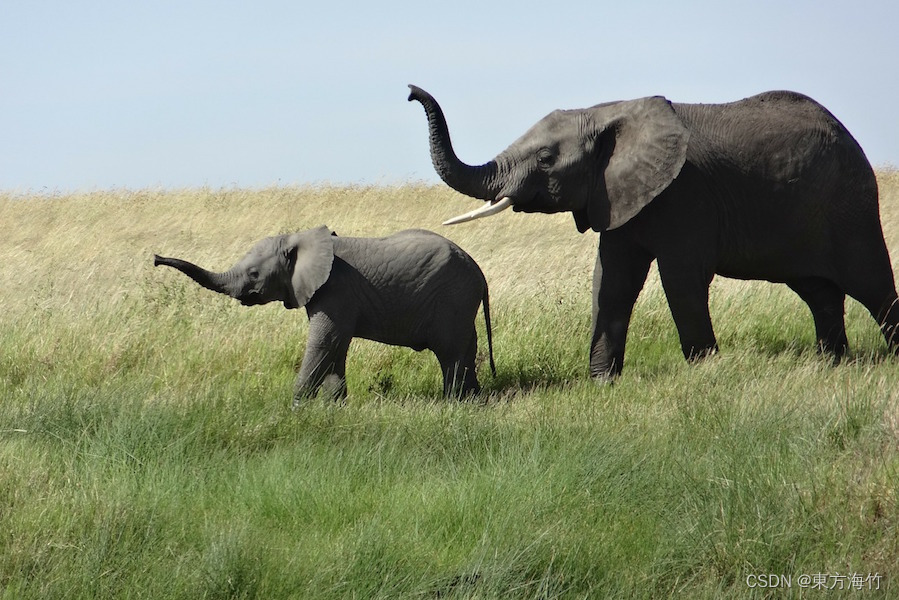
我们会用VGG16和下面这张图做一个简单的demo

加载一个完整的VGG16模型，终于

from keras.applications.vgg16 import VGG16
from keras import backend as K
# 如果你希望你编写的Keras模块与Theano(th)和TensorFlow(tf)兼容，
# 则必须通过抽象Keras后端API来编写
K.clear_session()

# 加载完整的VGG16模型
# Note that we are including the densely-connected classifier on top;
# all previous times, we were discarding it.
model = VGG16(weights='imagenet')

把原始图片一顿处理后predict一下

from keras.preprocessing import image
from keras.applications.vgg16 import preprocess_input, decode_predictions
import numpy as np

# The local path to our target image
img_path = 'D:\\tmp\\creative_commons_elephant.jpg'

# `img` is a PIL image of size 224x224
img = image.load_img(img_path, target_size=(224, 224))

# `x` is a float32 Numpy array of shape (224, 224, 3)
x = image.img_to_array(img)

# We add a dimension to transform our array into a "batch"
# of size (1, 224, 224, 3)
x = np.expand_dims(x, axis=0)

# 将进行颜色标准化
x = preprocess_input(x)

# 预测，并打印TOP3的分类
preds = model.predict(x)

一顿操作后得到最终的热力图heatmap

# This is the "african elephant" entry in the prediction vector
african_elephant_output = model.output[:, 386]

# The is the output feature map of the `block5_conv3` layer,
# the last convolutional layer in VGG16
last_conv_layer = model.get_layer('block5_conv3')

# This is the gradient of the "african elephant" class with regard to
# the output feature map of `block5_conv3`
grads = K.gradients(african_elephant_output, last_conv_layer.output)[0]

# This is a vector of shape (512,), where each entry
# is the mean intensity of the gradient over a specific feature map channel
pooled_grads = K.mean(grads, axis=(0, 1, 2))

# This function allows us to access the values of the quantities we just defined:
# `pooled_grads` and the output feature map of `block5_conv3`,
# given a sample image
iterate = K.function([model.input], [pooled_grads, last_conv_layer.output[0]])

# These are the values of these two quantities, as Numpy arrays,
# given our sample image of two elephants
pooled_grads_value, conv_layer_output_value = iterate([x])

# We multiply each channel in the feature map array
# by "how important this channel is" with regard to the elephant class
for i in range(512):
    conv_layer_output_value[:, :, i] *= pooled_grads_value[i]

# The channel-wise mean of the resulting feature map
# is our heatmap of class activation
heatmap = np.mean(conv_layer_output_value, axis=-1)
heatmap = np.maximum(heatmap, 0) # 小于0则设成0
heatmap /= np.max(heatmap) # 除最大值

使用OpenCV来将热力图与原图叠加

import cv2

# We use cv2 to load the original image
img = cv2.imread(img_path)

# We resize the heatmap to have the same size as the original image
heatmap = cv2.resize(heatmap, (img.shape[1], img.shape[0]))

# We convert the heatmap to RGB
heatmap = np.uint8(255 * heatmap)

# We apply the heatmap to the original image
heatmap = cv2.applyColorMap(heatmap, cv2.COLORMAP_JET)

# 0.4 here is a heatmap intensity factor
superimposed_img = heatmap * 0.4 + img

# Save the image to disk
cv2.imwrite('D:\\tmp\\elephant_cam.jpg', superimposed_img)

最终热力图完成

参考文章&图书

《Python深度学习》

系列文章

Keras深度学习入门（一）
Keras计算机视觉（二）
Keras文本和序列（三）
Keras深度学习高级（四）
Keras生成式学习（五）

@ 学必求其心得，业必贵其专精