前面已经练习过神经网络的相关代码，其实弄明白了你会发现深度学习其实是个黑盒，不论是TensorFlow还是pytorch都已经为我们封装好了，我们不需要理解深度学习如何实现，神经网络如何计算，这些都不用我们管，可能最需要我们自己操心的就是逻辑，我们自己算法的逻辑，即如何借助这些工具实现我们的想法。

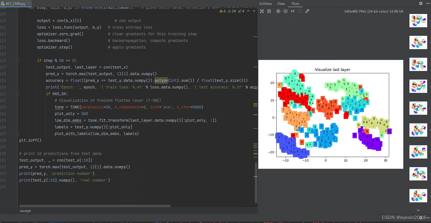
如下面这个cnn的例子，其实整个代码中关于神经网络的部分很少，几行代码就实现了，其余大部分都是在设计我们想要的东西。如各种指标，图像等

import os

# third-party library
import torch
import torch.nn as nn
import torch.utils.data as Data
import torchvision
import matplotlib.pyplot as plt

# torch.manual_seed(1)    # reproducible

# Hyper Parameters
EPOCH = 1               # train the training data n times, to save time, we just train 1 epoch
BATCH_SIZE = 50
LR = 0.001              # learning rate
DOWNLOAD_MNIST = True


# Mnist digits dataset
if not(os.path.exists('./mnist/')) or not os.listdir('./mnist/'):
    # not mnist dir or mnist is empyt dir
    DOWNLOAD_MNIST = True

train_data = torchvision.datasets.MNIST(
    root='./mnist/',
    train=True,                                     # this is training data
    transform=torchvision.transforms.ToTensor(),    # Converts a PIL.Image or numpy.ndarray to
                                                    # torch.FloatTensor of shape (C x H x W) and normalize in the range [0.0, 1.0]
    download=DOWNLOAD_MNIST,
)

# plot one example
print(train_data.train_data.size())                 # (60000, 28, 28)
print(train_data.train_labels.size())               # (60000)
plt.imshow(train_data.train_data[0].numpy(), cmap='gray')
plt.title('%i' % train_data.train_labels[0])
plt.show()

# Data Loader for easy mini-batch return in training, the image batch shape will be (50, 1, 28, 28)
train_loader = Data.DataLoader(dataset=train_data, batch_size=BATCH_SIZE, shuffle=True)

# pick 2000 samples to speed up testing
test_data = torchvision.datasets.MNIST(root='./mnist/', train=False)
test_x = torch.unsqueeze(test_data.test_data, dim=1).type(torch.FloatTensor)[:2000]/255.   # shape from (2000, 28, 28) to (2000, 1, 28, 28), value in range(0,1)
test_y = test_data.test_labels[:2000]


class CNN(nn.Module):
    def __init__(self):
        super(CNN, self).__init__()
        self.conv1 = nn.Sequential(         # input shape (1, 28, 28)
            nn.Conv2d(
                in_channels=1,              # input height
                out_channels=16,            # n_filters
                kernel_size=5,              # filter size
                stride=1,                   # filter movement/step
                padding=2,                  # if want same width and length of this image after Conv2d, padding=(kernel_size-1)/2 if stride=1
            ),                              # output shape (16, 28, 28)
            nn.ReLU(),                      # activation
            nn.MaxPool2d(kernel_size=2),    # choose max value in 2x2 area, output shape (16, 14, 14)
        )
        self.conv2 = nn.Sequential(         # input shape (16, 14, 14)
            nn.Conv2d(16, 32, 5, 1, 2),     # output shape (32, 14, 14)
            nn.ReLU(),                      # activation
            nn.MaxPool2d(2),                # output shape (32, 7, 7)
        )
        self.out = nn.Linear(32 * 7 * 7, 10)   # fully connected layer, output 10 classes

    def forward(self, x):
        x = self.conv1(x)
        x = self.conv2(x)
        x = x.view(x.size(0), -1)           # flatten the output of conv2 to (batch_size, 32 * 7 * 7)
        output = self.out(x)
        return output, x    # return x for visualization


cnn = CNN()
print(cnn)  # net architecture

optimizer = torch.optim.Adam(cnn.parameters(), lr=LR)   # optimize all cnn parameters
loss_func = nn.CrossEntropyLoss()                       # the target label is not one-hotted

# following function (plot_with_labels) is for visualization, can be ignored if not interested
from matplotlib import cm
try: from sklearn.manifold import TSNE; HAS_SK = True
except: HAS_SK = False; print('Please install sklearn for layer visualization')
def plot_with_labels(lowDWeights, labels):
    plt.cla()
    X, Y = lowDWeights[:, 0], lowDWeights[:, 1]
    for x, y, s in zip(X, Y, labels):
        c = cm.rainbow(int(255 * s / 9)); plt.text(x, y, s, backgroundcolor=c, fontsize=9)
    plt.xlim(X.min(), X.max()); plt.ylim(Y.min(), Y.max()); plt.title('Visualize last layer'); plt.show(); plt.pause(0.01)

plt.ion()
# training and testing
for epoch in range(EPOCH):
    for step, (b_x, b_y) in enumerate(train_loader):   # gives batch data, normalize x when iterate train_loader

        output = cnn(b_x)[0]               # cnn output
        loss = loss_func(output, b_y)   # cross entropy loss
        optimizer.zero_grad()           # clear gradients for this training step
        loss.backward()                 # backpropagation, compute gradients
        optimizer.step()                # apply gradients

        if step % 50 == 0:
            test_output, last_layer = cnn(test_x)
            pred_y = torch.max(test_output, 1)[1].data.numpy()
            accuracy = float((pred_y == test_y.data.numpy()).astype(int).sum()) / float(test_y.size(0))
            print('Epoch: ', epoch, '| train loss: %.4f' % loss.data.numpy(), '| test accuracy: %.2f' % accuracy)
            if HAS_SK:
                # Visualization of trained flatten layer (T-SNE)
                tsne = TSNE(perplexity=30, n_components=2, init='pca', n_iter=5000)
                plot_only = 500
                low_dim_embs = tsne.fit_transform(last_layer.data.numpy()[:plot_only, :])
                labels = test_y.numpy()[:plot_only]
                plot_with_labels(low_dim_embs, labels)
plt.ioff()

# print 10 predictions from test data
test_output, _ = cnn(test_x[:10])
pred_y = torch.max(test_output, 1)[1].data.numpy()
print(pred_y, 'prediction number')
print(test_y[:10].numpy(), 'real number')

所以这丰富的图像展示，以及数据指标的输出是需要我们自己有些功底去设计和实现的

CNN、RNN和全连接神经网络（FCN）在结构和工作原理上都有一些显著的区别：

结构和连接方式：

CNN使用卷积层和池化层来提取输入数据中的局部特征，并通过全连接层进行分类或回归。它通过在卷积核上滑动并在整个输入上执行卷积操作来捕捉特征。
RNN通过在时间步上的循环连接来处理序列数据，并在每个时间步上传递信息。RNN具有记忆功能，能够考虑到过去的上下文信息。
FCN是最简单的神经网络形式，它的每个神经元都与上一层的所有神经元相连接，没有明确的结构和连接模式。每个神经元都将输入的加权和传递给下一层。
参数共享：

CNN在卷积层中使用参数共享的概念，同一个卷积核在整个输入上进行滑动并提取特征，减少了网络的参数量。
RNN在每个时间步上都使用相同的权重参数，使得网络能够对不同时间步的输入共享相同的信息。
FCN中的每个神经元都有自己独立的权重参数，没有参数共享的概念。
数据处理方式：

CNN主要用于处理具有网格结构的数据，如图像。它通过卷积操作在局部区域上提取特征，并通过池化操作减小特征图的尺寸。
RNN适用于处理序列数据，如文本、语音等。它在每个时间步上接收输入，并传递隐状态，以捕捉时序信息和上下文关系。
FCN没有对特定数据类型进行假设，适用于任意结构的输入数据。
应用领域：

CNN广泛应用于计算机视觉任务，如图像分类、目标检测和图像生成等。
RNN在自然语言处理（NLP）领域中得到广泛应用，如语言建模、机器翻译和情感分析等。
FCN在某些简单任务或特定需求的情况下使用，但在处理复杂数据结构或序列数据时效果有限。

总之，CNN、RNN和FCN是深度学习中常用的神经网络架构，它们在结构、连接方式和适用领域上有所不同，可以根据具体的任务和数据类型选择合适的网络结构。

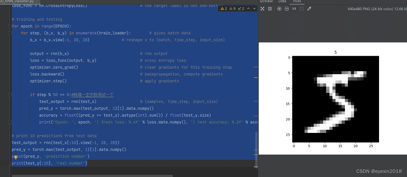
看一下RNN的分类应用代码，这里用LSTM实现

import torch
from torch import nn
import torchvision.datasets as dsets
import torchvision.transforms as transforms
import matplotlib.pyplot as plt


# torch.manual_seed(1)    # reproducible

# Hyper Parameters
EPOCH = 1               # train the training data n times, to save time, we just train 1 epoch
BATCH_SIZE = 64
TIME_STEP = 28          # rnn time step / image height
INPUT_SIZE = 28         # rnn input size / image width
LR = 0.01               # learning rate
DOWNLOAD_MNIST = True   # set to True if haven't download the data


# Mnist digital dataset
train_data = dsets.MNIST(
    root='./mnist/',
    train=True,                         # this is training data
    transform=transforms.ToTensor(),    # Converts a PIL.Image or numpy.ndarray to
                                        # torch.FloatTensor of shape (C x H x W) and normalize in the range [0.0, 1.0]
    download=DOWNLOAD_MNIST,            # download it if you don't have it
)

# plot one example
print(train_data.train_data.size())     # (60000, 28, 28)
print(train_data.train_labels.size())   # (60000)
plt.imshow(train_data.train_data[0].numpy(), cmap='gray')
plt.title('%i' % train_data.train_labels[0])
plt.show()

# Data Loader for easy mini-batch return in training
train_loader = torch.utils.data.DataLoader(dataset=train_data, batch_size=BATCH_SIZE, shuffle=True)

# convert test data into Variable, pick 2000 samples to speed up testing
test_data = dsets.MNIST(root='./mnist/', train=False, transform=transforms.ToTensor())
test_x = test_data.test_data.type(torch.FloatTensor)[:2000]/255.   # shape (2000, 28, 28) value in range(0,1)
test_y = test_data.test_labels.numpy()[:2000]    # covert to numpy array


class RNN(nn.Module):
    def __init__(self):
        super(RNN, self).__init__()

        self.rnn = nn.LSTM(         # if use nn.RNN(), it hardly learns,lstm
            input_size=INPUT_SIZE,
            hidden_size=64,         # rnn hidden unit
            num_layers=1,           # number of rnn layer
            batch_first=True,       # input & output will has batch size as 1s dimension. e.g. (batch, time_step, input_size)
        )

        self.out = nn.Linear(64, 10)

    def forward(self, x):
        # x shape (batch, time_step, input_size)
        # r_out shape (batch, time_step, output_size)
        # h_n shape (n_layers, batch, hidden_size)
        # h_c shape (n_layers, batch, hidden_size)
        r_out, (h_n, h_c) = self.rnn(x, None)#r_out表示从RNN层获得的输出。[:, -1, :]表示从r_out中选取所有样本（:），最后一个时间步（-1），以及所有特征维度（:）的部分。

        out = self.out(r_out[:, -1, :])
        return out


rnn = RNN()
print(rnn)

optimizer = torch.optim.Adam(rnn.parameters(), lr=LR)   # optimize all cnn parameters
loss_func = nn.CrossEntropyLoss()                       # the target label is not one-hotted

# training and testing
for epoch in range(EPOCH):
    for step, (b_x, b_y) in enumerate(train_loader):        # gives batch data
        b_x = b_x.view(-1, 28, 28)              # reshape x to (batch, time_step, input_size)

        output = rnn(b_x)                               # rnn output
        loss = loss_func(output, b_y)                   # cross entropy loss
        optimizer.zero_grad()                           # clear gradients for this training step
        loss.backward()                                 # backpropagation, compute gradients
        optimizer.step()                                # apply gradients

        if step % 50 == 0:#每隔一定步数测试一下
            test_output = rnn(test_x)                   # (samples, time_step, input_size)
            pred_y = torch.max(test_output, 1)[1].data.numpy()
            accuracy = float((pred_y == test_y).astype(int).sum()) / float(test_y.size)
            print('Epoch: ', epoch, '| train loss: %.4f' % loss.data.numpy(), '| test accuracy: %.2f' % accuracy)

# print 10 predictions from test data
test_output = rnn(test_x[:10].view(-1, 28, 28))
pred_y = torch.max(test_output, 1)[1].data.numpy()
print(pred_y, 'prediction number')
print(test_y[:10], 'real number')

准确率逐渐提高

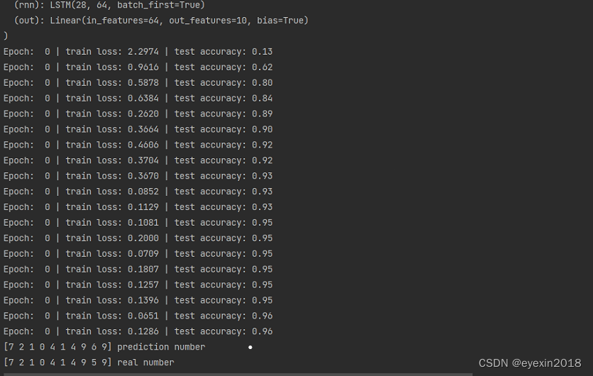
同时打印出了一个示例

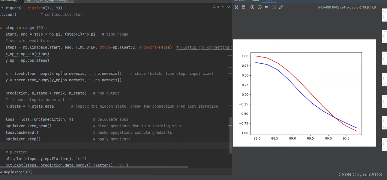
再看看RNN的回归应用代码

import torch
from torch import nn
import numpy as np
import matplotlib.pyplot as plt

# torch.manual_seed(1)    # reproducible

# Hyper Parameters
TIME_STEP = 10      # rnn time step
INPUT_SIZE = 1      # rnn input size
LR = 0.02           # learning rate

# show data
steps = np.linspace(0, np.pi*2, 100, dtype=np.float32)  # float32 for converting torch FloatTensor
x_np = np.sin(steps)
y_np = np.cos(steps)
plt.plot(steps, y_np, 'r-', label='target (cos)')
plt.plot(steps, x_np, 'b-', label='input (sin)')
plt.legend(loc='best')
plt.show()


class RNN(nn.Module):
    def __init__(self):
        super(RNN, self).__init__()

        self.rnn = nn.RNN(
            input_size=INPUT_SIZE,
            hidden_size=32,     # rnn hidden unit
            num_layers=1,       # number of rnn layer
            batch_first=True,   # input & output will has batch size as 1s dimension. e.g. (batch, time_step, input_size)
        )
        self.out = nn.Linear(32, 1)

    def forward(self, x, h_state):
        # x (batch, time_step, input_size)
        # h_state (n_layers, batch, hidden_size)
        # r_out (batch, time_step, hidden_size)
        r_out, h_state = self.rnn(x, h_state)

        outs = []    # save all predictions
        for time_step in range(r_out.size(1)):    # calculate output for each time step
            outs.append(self.out(r_out[:, time_step, :]))
        return torch.stack(outs, dim=1), h_state

        # instead, for simplicity, you can replace above codes by follows
        # r_out = r_out.view(-1, 32)
        # outs = self.out(r_out)
        # outs = outs.view(-1, TIME_STEP, 1)
        # return outs, h_state
        
        # or even simpler, since nn.Linear can accept inputs of any dimension 
        # and returns outputs with same dimension except for the last
        # outs = self.out(r_out)
        # return outs

rnn = RNN()
print(rnn)

optimizer = torch.optim.Adam(rnn.parameters(), lr=LR)   # optimize all cnn parameters
loss_func = nn.MSELoss()

h_state = None      # for initial hidden state

plt.figure(1, figsize=(12, 5))
plt.ion()           # continuously plot

for step in range(100):
    start, end = step * np.pi, (step+1)*np.pi   # time range
    # use sin predicts cos
    steps = np.linspace(start, end, TIME_STEP, dtype=np.float32, endpoint=False)  # float32 for converting torch FloatTensor
    x_np = np.sin(steps)
    y_np = np.cos(steps)

    x = torch.from_numpy(x_np[np.newaxis, :, np.newaxis])    # shape (batch, time_step, input_size)
    y = torch.from_numpy(y_np[np.newaxis, :, np.newaxis])

    prediction, h_state = rnn(x, h_state)   # rnn output
    # !! next step is important !!
    h_state = h_state.data        # repack the hidden state, break the connection from last iteration

    loss = loss_func(prediction, y)         # calculate loss
    optimizer.zero_grad()                   # clear gradients for this training step
    loss.backward()                         # backpropagation, compute gradients
    optimizer.step()                        # apply gradients

    # plotting
    plt.plot(steps, y_np.flatten(), 'r-')
    plt.plot(steps, prediction.data.numpy().flatten(), 'b-')
    plt.draw(); plt.pause(0.05)

plt.ioff()
plt.show()

这里就直接用RNN实现了。结果如下

多练多敲代码，不必要求一遍就全部理解全都掌握，这是不可能的，重要的是多次练习逐渐领悟