💡 作者:韩信子@ShowMeAI
📘 数据分析实战系列:https://www.showmeai.tech/tutorials/40
📘 机器学习实战系列:https://www.showmeai.tech/tutorials/41
📘 本文地址:https://www.showmeai.tech/article-detail/401
📢 声明:版权所有,转载请联系平台与作者并注明出处
📢 收藏ShowMeAI查看更多精彩内容
💡 引言

在过去几年中,客户对航空公司的满意度一直在稳步攀升。在 COVID-19 大流行导致的停顿之后,航空旅行业重新开始,大家越来越关注航空出行的满意度问题,客户也会对一些常见问题,如『不舒服的座位』、『拥挤的空间』、『延误』和『不合标准的设施』等进行反馈。
各家航空公司也越来越关注客户满意度问题并努力提高。对航空公司而言,出色的客户服务,是销量和客户留存的关键;反之,糟糕的客户服务评级会导致客户流失和公司声誉不佳。

在本项目中,我们将对航空满意度数据进行分析建模,对满意度进行预估,并找出影响满意度的核心因素。
💡 数据&环境
这里使用到的主要开发环境是 Jupyter Notebooks,基于 Python 3.9 完成。依赖的工具库包括 用于数据探索分析的Pandas、Numpy、Seaborn 和 Matplotlib 库、用于建模和优化的 XGBoost 和 Scikit-Learn 库,以及用于模型可解释性分析的 SHAP 工具库。

关于以上工具库的用法,ShowMeAI在实战文章中做了详细介绍,大家可以查看以下教程系列和文章
📘数据分析实战:Python 数据分析实战教程
📘机器学习实战:手把手教你玩转机器学习系列
📘基于SHAP的机器学习可解释性实战

我们本次用到的数据集是 🏆Kaggle航空满意度数据集。数据集使用csv格式文件存储,预先切分好了 80% 的训练集 和 20% 的测试集;目标列“*Satisfaction/*满意度”。大家可以通过 ShowMeAI 的百度网盘地址下载。
🏆 实战数据集下载(百度网盘):公众号『ShowMeAI研究中心』回复『实战』,或者点击 这里 获取本文 [36]『航班乘客满意度』场景数据分析建模与业务归因解释 『Airline Passenger Satisfaction数据集』
⭐ ShowMeAI官方GitHub:https://github.com/ShowMeAI-Hub
详细的数据列字段如下:
| 字段 | 说明 | 详情 |
|---|---|---|
| Gender | 乘客性别 | Female, Male |
| Customer Type | 乘客类型 | Loyal customer, disloyal customer |
| Age | 乘客年龄 | – |
| Type of Travel | 乘客出行目的 | Personal Travel, Business Travel |
| Class | 客舱等级 | Business, Eco, Eco Plus |
| Flight distance | 航程距离 | – |
| Inflight wifi service | 机上WiFi服务满意度 | 0:Not Applicable;1-5 |
| Departure/Arrival time convenient | 起飞/降落舒适度满意度 | – |
| Ease of Online booking | 在线预定满意度 | – |
| Gate location | 登机门位置满意度 | – |
| Food and drink | 机上食物满意度 | – |
| Online boarding | 在线值机满意度 | – |
| Seat comfort | 座椅舒适度满意度 | – |
| Inflight entertainment | 机上娱乐设施满意度 | – |
| On-board service | 登机服务满意度 | – |
| Leg room service | 腿部空间满意度 | – |
| Baggage handling | 行李处理满意度 | – |
| Check-in service | 值机满意度 | – |
| Inflight service | 机上服务满意度 | – |
| Cleanliness | 环境干净度满意度 | – |
| Departure Delay in Minutes | 起飞延误时间 | – |
| Arrival Delay in Minutes | 抵达延误时间 | – |
| Satisfaction | 航线满意度 | Satisfaction, neutral or dissatisfaction |
💡 数据一览和清理
💦 数据一览
我们先导入工具库,进行基本的设定,并读取数据。
# 导入工具库
import pandas as pd
import numpy as np
import scipy.stats as sp
import matplotlib.pyplot as plt
import seaborn as sns
import warnings
warnings.filterwarnings("ignore")
# 可视化图例设定
from matplotlib import rcParams
# 字体大小
rcParams['font.size'] = 12
# 图例大小
rcParams['figure.figsize'] = 7, 5
# 读取数据
air_train_df = pd.read_csv('air-train.csv')
air_test_df = pd.read_csv('air-test.csv')
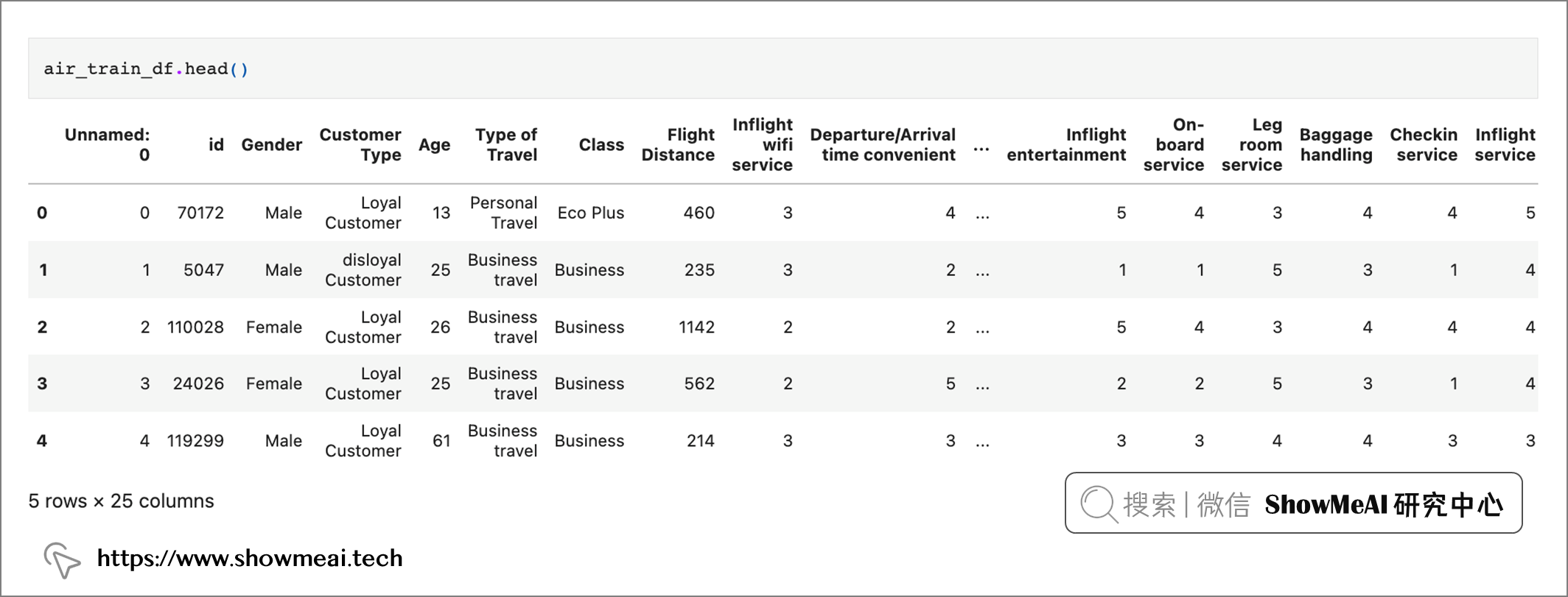
air_train_df.head()
air_train_df.satisfaction.value_counts()
neutral or dissatisfied    58879
satisfied                  45025
Name: satisfaction, dtype: int64
air_train_df.info()

air_test_df.info()
输出的数据信息如下,我们使用到的数据总共包含 129,880 行25 列。数据集被预拆分为包含 103,904 行的训练数据集(19.8MB)和包含 25,976 行的测试数据集(5MB)。
Training Data Set (air_train_df):
<class 'pandas.core.frame.DataFrame'>
RangeIndex: 103904 entries, 0 to 103903
Data columns (total 25 columns):
 #   Column                             Non-Null Count   Dtype
---  ------                             --------------   -----
 0   Unnamed: 0                         103904 non-null  int64
 1   id                                 103904 non-null  int64
 2   Gender                             103904 non-null  object
 3   Customer Type                      103904 non-null  object
 4   Age                                103904 non-null  int64
 5   Type of Travel                     103904 non-null  object
 6   Class                              103904 non-null  object
 7   Flight Distance                    103904 non-null  int64
 8   Inflight wifi service              103904 non-null  int64
 9   Departure/Arrival time convenient  103904 non-null  int64
 10  Ease of Online booking             103904 non-null  int64
 11  Gate location                      103904 non-null  int64
 12  Food and drink                     103904 non-null  int64
 13  Online boarding                    103904 non-null  int64
 14  Seat comfort                       103904 non-null  int64
 15  Inflight entertainment             103904 non-null  int64
 16  On-board service                   103904 non-null  int64
 17  Leg room service                   103904 non-null  int64
 18  Baggage handling                   103904 non-null  int64
 19  Checkin service                    103904 non-null  int64
 20  Inflight service                   103904 non-null  int64
 21  Cleanliness                        103904 non-null  int64
 22  Departure Delay in Minutes         103904 non-null  int64
 23  Arrival Delay in Minutes           103594 non-null  float64
 24  satisfaction                       103904 non-null  object
dtypes: float64(1), int64(19), object(5)
memory usage: 19.8+ MB

Testing Set (air_test_df):
<class 'pandas.core.frame.DataFrame'>
RangeIndex: 25976 entries, 0 to 25975
Data columns (total 25 columns):
 #   Column                             Non-Null Count  Dtype
---  ------                             --------------  -----
 0   Unnamed: 0                         25976 non-null  int64
 1   id                                 25976 non-null  int64
 2   Gender                             25976 non-null  object
 3   Customer Type                      25976 non-null  object
 4   Age                                25976 non-null  int64
 5   Type of Travel                     25976 non-null  object
 6   Class                              25976 non-null  object
 7   Flight Distance                    25976 non-null  int64
 8   Inflight wifi service              25976 non-null  int64
 9   Departure/Arrival time convenient  25976 non-null  int64
 10  Ease of Online booking             25976 non-null  int64
 11  Gate location                      25976 non-null  int64
 12  Food and drink                     25976 non-null  int64
 13  Online boarding                    25976 non-null  int64
 14  Seat comfort                       25976 non-null  int64
 15  Inflight entertainment             25976 non-null  int64
 16  On-board service                   25976 non-null  int64
 17  Leg room service                   25976 non-null  int64
 18  Baggage handling                   25976 non-null  int64
 19  Checkin service                    25976 non-null  int64
 20  Inflight service                   25976 non-null  int64
 21  Cleanliness                        25976 non-null  int64
 22  Departure Delay in Minutes         25976 non-null  int64
 23  Arrival Delay in Minutes           25893 non-null  float64
 24  satisfaction                       25976 non-null  object
dtypes: float64(1), int64(19), object(5)
memory usage: 5.0+ MB
数据集中,19 个 int 数据类型字段,1 个 float 数据类型字段,5 个分类数据类型(对象)字段。
💦 数据清洗
下面我们进行数据清洗:
id和unnamed两列没有作用,我们直接删除。- 『到达延误时间』列是浮点数据类型,『出发延误时间』列是整数数据类型,在进行进一步分析前,我们把它们都调整为浮点数类型,保持一致。
- 类别型变量,包括列名和列取值,我们对它们做规范化处理(全部小写化,以便在后续建模过程中准确编码)。
Arrival Delay列中也存在缺失值——训练集中缺少 310 个,测试集中缺少 83 个。我们在这里用最简单的平均值来填充它们。- 数据集的满意度等级列应该是 1 到 5 的等级评分。有一些取值为0的脏数据,我们剔除掉它们。
- 我们把航班延误信息聚合成一些统一的列。表明航班是否经历了延误(起飞或到达)和航班延误所花费的总时间。
def clean_data(orig_df):
    '''
    This function applies 5 steps to the dataframe to clean the data.
    1. Dropping of unnecessary columns
    2. Uniformize datatypes in delay column
    3. Normalizing column names.
    4. Normalizing text values in columns.
    5. Imputing numeric null values with the mean value of the column.
    6. Dropping "zero" values from ranked categorical variables.
    7. Creating aggregated flight delay column


    Return: Cleaned DataFrame, ready for analysis - final encoding still to be applied.
    '''

    df = orig_df.copy()

    '''1. Dropping off unnecessary columns'''
    df.drop(['Unnamed: 0', 'id'], axis = 1, inplace = True)

    '''2. Uniformizing datatype in delay column'''
    df['Departure Delay in Minutes'] = df['Departure Delay in Minutes'].astype(float)

    '''3. Normalizing column names'''
    df.columns = df.columns.str.lower()

    '''Replacing spaces and other characters with underscores, this is more
    for us to make it easier to work with them and so that we can call them using dot notation.'''
    special_chars = "/ -"
    for special_char in special_chars:
        df.columns = [col.replace(special_char, '_') for col in df.columns]

    '''4. Normalizing text values in columns'''
    cat_cols = ['gender', 'customer_type', 'class', 'type_of_travel', 'satisfaction']

    for column in cat_cols:
        df[column] = df[column].str.lower()

    '''5. Imputing the nulls in the arrival delay column with the mean.
    Since we cannot safely equate these nulls to a zero value, the mean value of the column is the
    most sensible method of replacement.'''
    df['arrival_delay_in_minutes'].fillna(df['arrival_delay_in_minutes'].mean(), inplace = True)
    df.round({'arrival_delay_in_minutes' : 1})

    '''6. Dropping rows from ranked value columns where "zero" exists as a value
    Since these columns are meant to be ranked on a scale from 1 to 5, having zero as a value
    does not make sense nor does it help us in any way.'''
    rank_list = ["inflight_wifi_service", "departure_arrival_time_convenient", "ease_of_online_booking", "gate_location",
                "food_and_drink", "online_boarding", "seat_comfort", "inflight_entertainment", "on_board_service",
                "leg_room_service", "baggage_handling", "checkin_service", "inflight_service", "cleanliness"]

    '''7. Creating aggregated and categorical flight delay columns'''
    df['total_delay_time'] = (df['departure_delay_in_minutes'] + df['arrival_delay_in_minutes'])
    df['was_flight_delayed'] = np.nan
    df['was_flight_delayed'] = np.where(df['total_delay_time'] > 0, 'yes', 'no')

    for col in rank_list:
        df.drop(df.loc[df[col]==0].index, inplace=True)

    cleaned_df = df

    return cleaned_df
💡 探索性分析
完成数据加载与基本的数据清洗后,我们对数据进行进一步的分析挖掘,即EDA(探索性数据分析)的过程。
💦 目标变量(客户满意度)分布如何
我们先对目标变量进行分析,即客户满意度情况,这是建模的最终标签,它是一个类别型字段。
air_train_cleaned = clean_data(air_train_df)
air_test_cleaned = clean_data(air_test_df)

fig = plt.figure(figsize = (10,7))
air_train_cleaned.satisfaction.value_counts(normalize = True).plot(kind='bar', alpha = 0.9, rot=0)
plt.title('Customer satisfaction')
plt.ylabel('Percent')
plt.show()
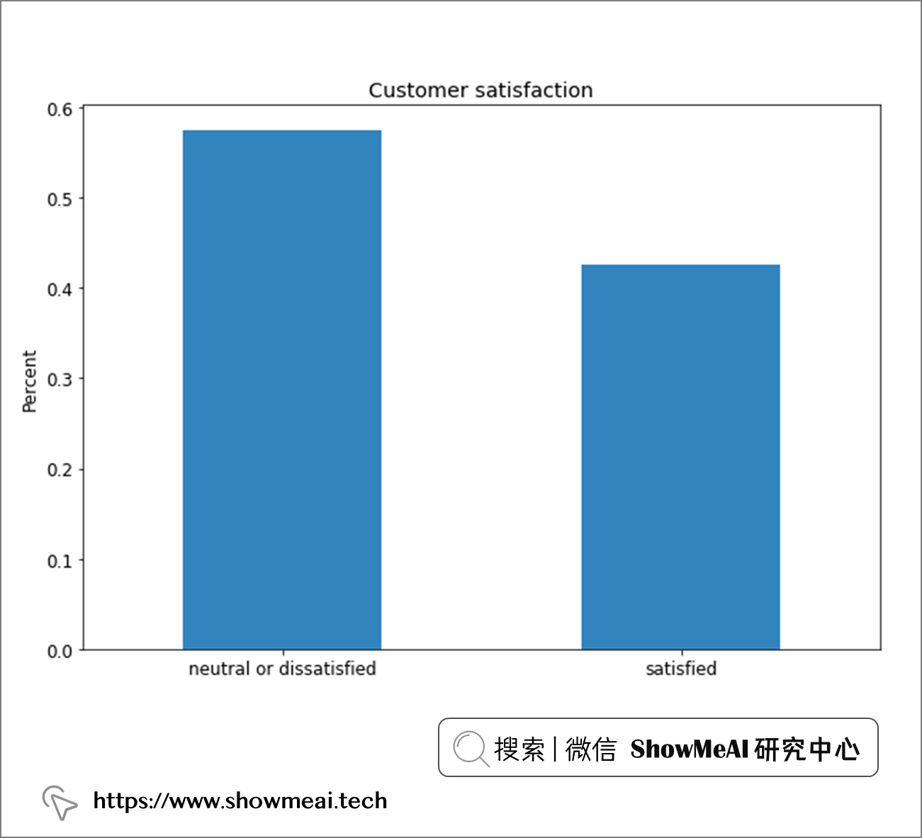
总体来说,标签还算均衡,大约 55% 的中立或不满意,45% 的满意。这种标签比例分布下,我们不需要进行数据采样。
💦 性别和客户身份 V.S. 满意度
with sns.axes_style(style = 'ticks'):
    d = sns.histplot(x = "gender",  hue= 'satisfaction', data = air_train_cleaned,
                     stat = 'percent', multiple="dodge", palette = 'Set1')
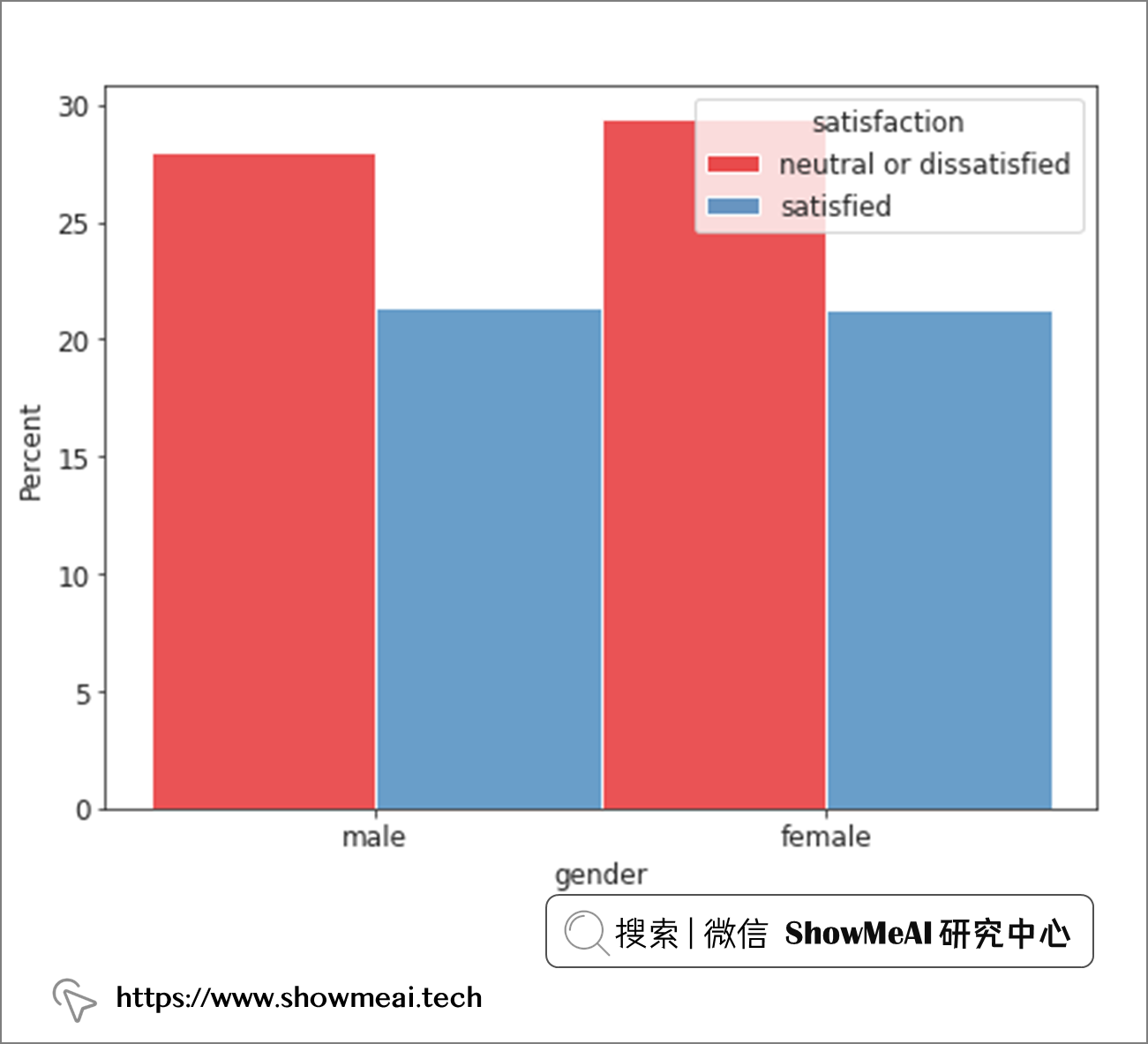
从性别维度来看,男女似乎差别不大,总体满意度可能更取决于其他因素。
with sns.axes_style(style = 'ticks'):
    d = sns.histplot(x = "customer_type",  hue= 'satisfaction', data = air_train_cleaned,
                     stat = 'percent', multiple="dodge", palette = 'Set1')
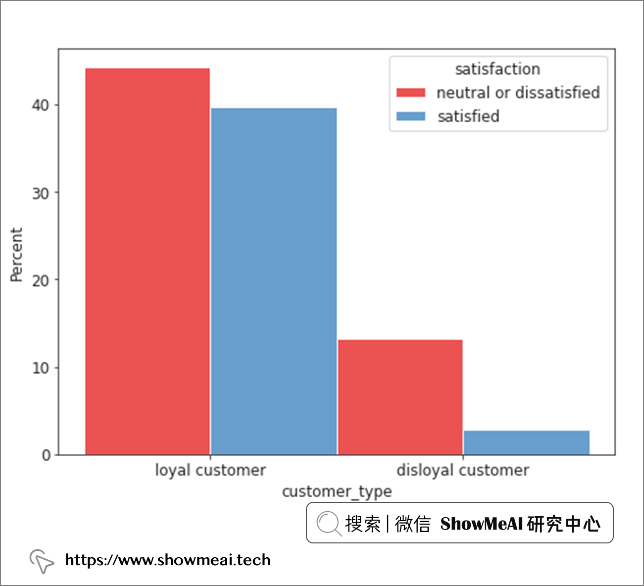
从客户忠诚度角度看,忠诚客户的满意度比例会相对高一点,这也是我们可以直观理解的。
💦 客舱等级 V.S. 满意度
with sns.axes_style(style = 'ticks'):
    d = sns.histplot(x = "class",  hue= 'satisfaction', data = air_train_cleaned,
                     stat = 'percent', multiple="dodge", palette = 'Set1')
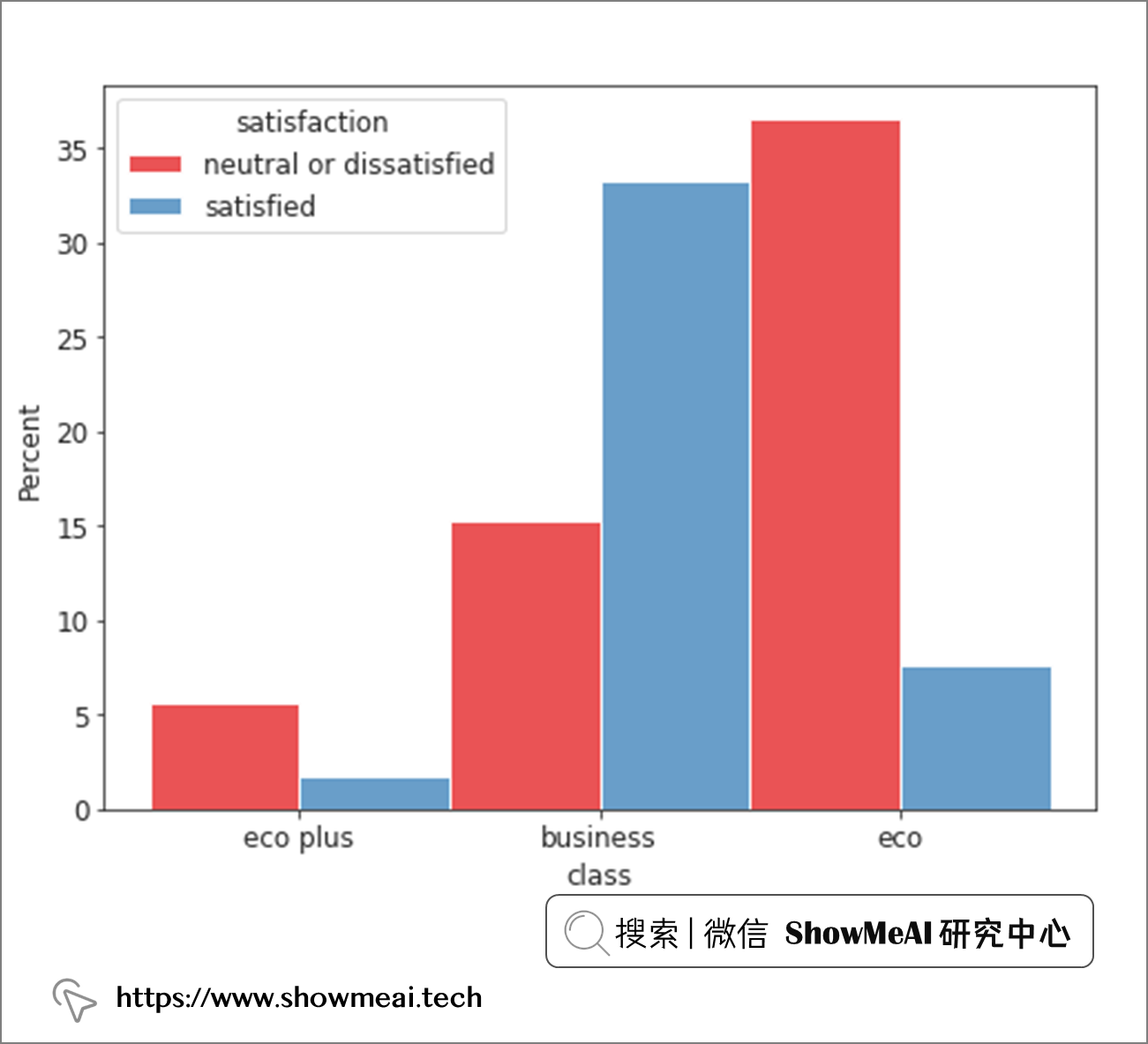
我们分别看一下乘坐经济舱、高级舱和商务舱的旅客的满意度,从上面的分布我们可以观察到乘坐高级舱(商务舱)的乘客与乘坐长途客舱(经济舱或豪华舱)的乘客在满意度上存在根本差异。
那我们进而看一下因个人休闲而出差的乘客
with sns.axes_style(style = 'ticks'):
    d = sns.histplot(x = "type_of_travel",  hue= 'satisfaction', data = air_train_cleaned,
                     stat = 'percent', multiple="dodge", palette = 'Set1')
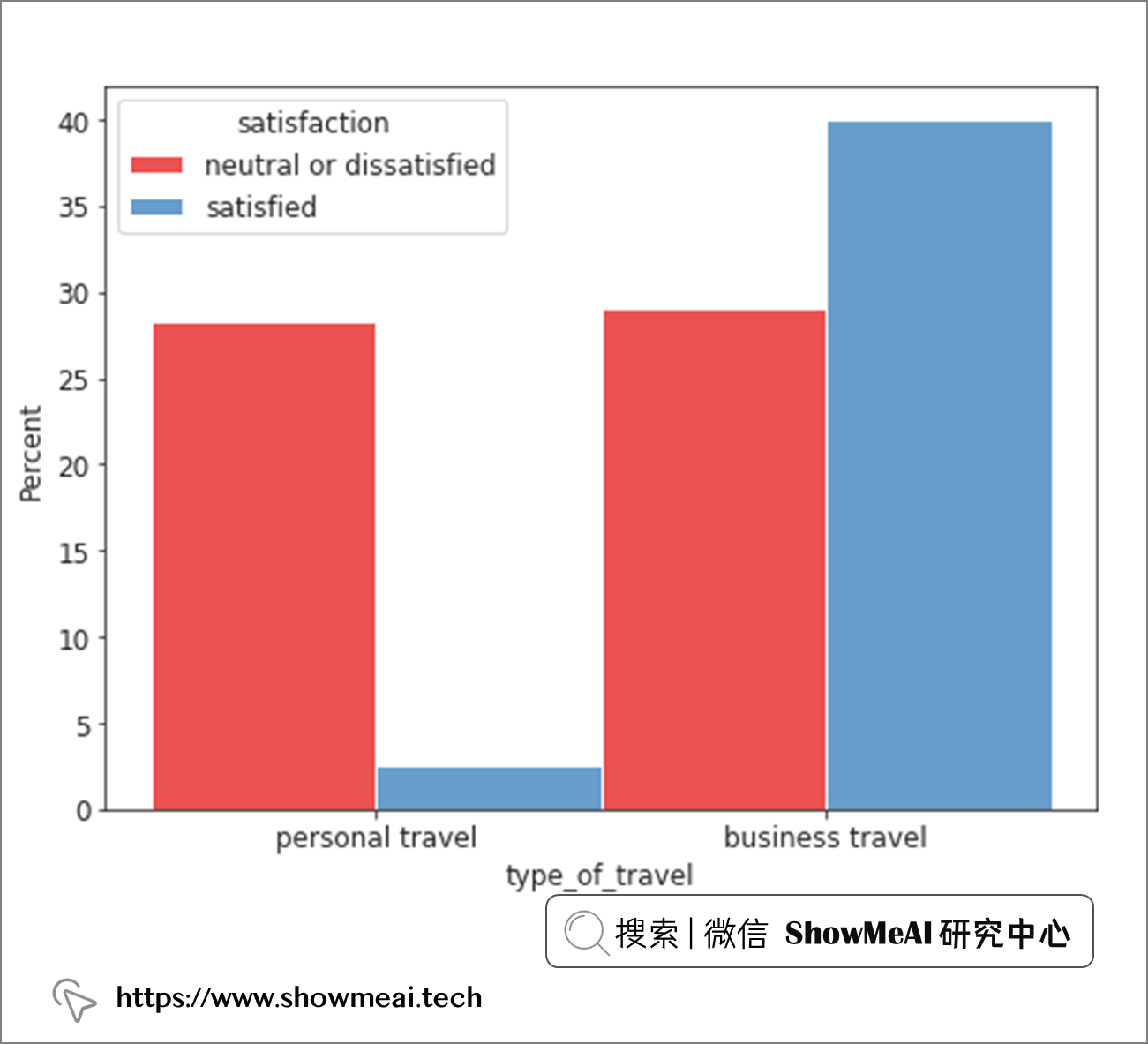
从上面的分析我们发现,商务旅行的乘客与休闲旅行的乘客之间的满意度存在非常显著的差异。
💦 年龄段 V.S. 满意度
with sns.axes_style('white'):
    g = sns.catplot(x = 'age', data = air_train_cleaned,
                    kind = 'count', hue = 'satisfaction', order = range(7, 80),
                    height = 8.27, aspect=18.7/8.27, legend = False,
                   palette = 'Set1')

plt.legend(loc='upper right');
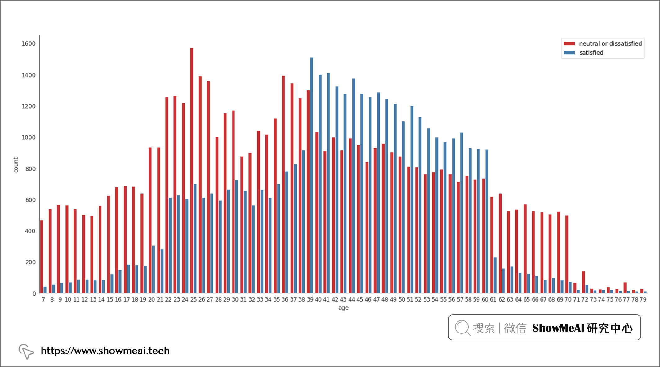
sns.violinplot(data = air_train_cleaned, x = "satisfaction", y = "age", palette='Set1')

上图是年龄和满意度之间的关系,分析结果非常有趣,37-61 岁年龄组与其他年龄组之间存在显著差异(他们对体验的满意度远远高于其他组的乘客)。另外我们还观察到,这个段的乘客的满意度随着年龄的增长而稳步上升。
💦 飞行时间长短 V.S. 满意度
sns.violinplot(data = air_train_cleaned, x = "satisfaction", y = "flight_distance", palette = 'Set1')
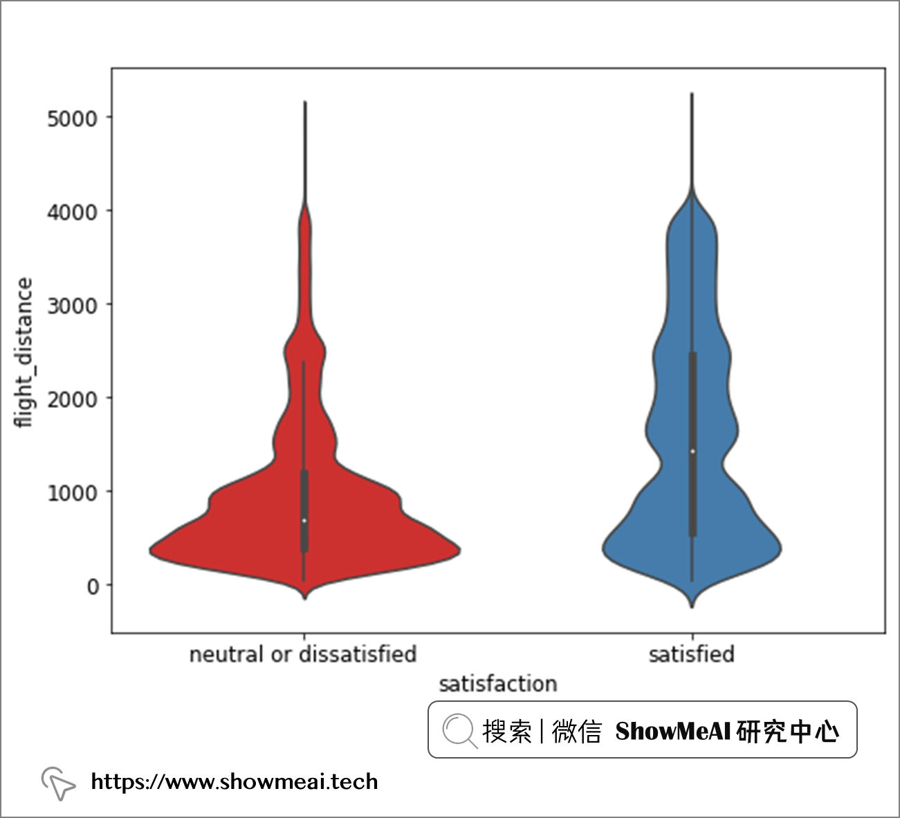
从飞行距离维度,我们看不出显著的满意度差异,而且绝大多数乘客的航班航程为 1,000 英里或更短。
💦 飞行距离 V.S. 各个体验维度
score_cols = ["inflight_wifi_service", "departure_arrival_time_convenient", "ease_of_online_booking",
              "gate_location","food_and_drink", "online_boarding", "seat_comfort", "inflight_entertainment",
              "on_board_service","leg_room_service", "baggage_handling", "checkin_service", "inflight_service","cleanliness"]
plt.figure(figsize=(40, 20))
plt.subplots_adjust(hspace=0.3)

# Loop through scored columns
for n, score_col in enumerate(score_cols):
    # Add a new subplot iteratively
    ax = plt.subplot(4, 4, n + 1)

    # Filter df and plot scored column on new axis
    sns.violinplot(data = air_train_cleaned,
                   x = score_col,
                   y = 'flight_distance',
                   hue = "satisfaction",
                   split = True,
                   ax = ax,
                   palette = 'Set1')

    # Chart formatting
    ax.set_title(score_col)
    ax.legend(loc='upper center', bbox_to_anchor=(0.5, -0.05),
          fancybox=True, shadow=True, ncol=5)
    ax.set_xlabel("")

我们使用小提琴图对航班不同飞行距离和旅客对不同服务维度评级的满意程度进行交叉分析如上,飞行距离对客户满意度的影响还是比较大的。
💦 年龄 V.S. 各个体验维度
plt.figure(figsize=(40, 20))
plt.subplots_adjust(hspace=0.3)

# Loop through scored columns
for n, score_col in enumerate(score_cols):
    # Add a new subplot iteratively
    ax = plt.subplot(4, 4, n + 1)

    # Filter df and plot scored column on new axis
    sns.violinplot(data = air_train_cleaned,
                   x = score_col,
                   y = 'age',
                   hue = "satisfaction",
                   split = True,
                   ax = ax,
                   palette = 'Set1')

    # Chart formatting
    ax.set_title(score_col),
    ax.legend(loc='upper center', bbox_to_anchor=(0.5, -0.05),
          fancybox=True, shadow=True, ncol=5)
    ax.set_xlabel("")

同样的方式,我们针对不同的年龄段,对于乘客在不同维度的体验满意度分析如上,我们观察到,在这些分布的大多数中,37-60 岁年龄组有一个明显的高峰。
💦 客舱等级和出行目的 V.S. 各个体验维度
plt.figure(figsize=(40, 20))
plt.subplots_adjust(hspace=0.3)

# Loop through scored columns
for n, score_col in enumerate(score_cols):
    # Add a new subplot iteratively
    ax = plt.subplot(4, 4, n + 1)

    # Filter df and plot scored column on new axis
    sns.violinplot(data = air_train_cleaned,
                   x = 'class',
                   y = score_col,
                   hue = "satisfaction",
                   split = True,
                   ax = ax,
                   palette = 'Set1')

    # Chart formatting
    ax.set_title(score_col)
    ax.legend(loc='upper center', bbox_to_anchor=(0.5, -0.05),
          fancybox=True, shadow=True, ncol=5)
    ax.set_xlabel("")

plt.figure(figsize=(40, 20))
plt.subplots_adjust(hspace=0.3)

# Loop through scored columns
for n, score_col in enumerate(score_cols):
    # Add a new subplot iteratively
    ax = plt.subplot(4, 4, n + 1)

    # Filter df and plot scored column on new axis
    sns.violinplot(data = air_train_cleaned,
                   x = 'type_of_travel',
                   y = score_col,
                   hue = "satisfaction",
                   split = True,
                   ax = ax,
                   palette = 'Set1')

    # Chart formatting
    ax.set_title(score_col)
    ax.legend(loc='upper center', bbox_to_anchor=(0.5, -0.05),
          fancybox=True, shadow=True, ncol=5)
    ax.set_xlabel("")
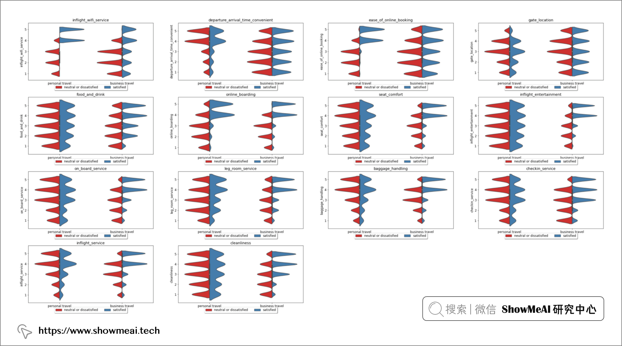
同样的方式,我们针对不同的客舱等级和出行目的,对于乘客在不同维度的体验满意度分析如上,我们观察到,这两个信息很大程度影响乘客满意度。机上 Wi-Fi 服务、在线登机、座椅舒适度、机上娱乐、机上客户服务、腿部空间和机上客户服务的满意度和不满意度都出现了明显的高峰。
很有意思的一点是机上wi-fi服务栏,这一项的满意似乎对乘坐经济舱和经济舱的客户的航班行程满意有很大影响,但它似乎对商务舱旅客的满意度没有太大影响。
💡 数据处理和特征选择
💦 数据处理/特征工程
在将数据引入模型之前,必须对数据进行编码以便为建模做好准备。我们针对类别型的变量,使用序号编码进行编码映射,具体代码如下(考虑到下面的不同类别取值本身有程度大小关系,以及我们会使用xgboost等非线性模型,因此序号编码是OK的)
关于特征工程的详细知识,欢迎大家查看ShowMeAI的系列教程文章:
📘机器学习实战 | 机器学习特征工程最全解读
from sklearn.preprocessing import OrdinalEncoder

def encode_data(orig_df):
    '''
    Encodes remaining categorical variables of data frame to be ready for model ingestion

    Inputs:
       Dataframe

    Manipulations:
        Encoding of categorical variables.

    Return:
        Encoded Column Values
    '''

    df = orig_df.copy()

    #Ordinal encode of scored rating columns.
    encoder = OrdinalEncoder()

    for j in score_cols:
        df[j] = encoder.fit_transform(df[[j]])

    # Replacement of binary categories.
    df.was_flight_delayed.replace({'no': 0, 'yes' : 1}, inplace = True)
    df['satisfaction'].replace({'neutral or dissatisfied': 0, 'satisfied': 1},inplace = True)
    df.customer_type.replace({'disloyal customer': 0, 'loyal customer': 1}, inplace = True)
    df.type_of_travel.replace({'personal travel': 0, 'business travel': 1}, inplace = True)
    df.gender.replace({'male': 0, 'female' : 1}, inplace = True)

    encoded_df = pd.get_dummies(df, columns = ['class'])

    return encoded_df
# 对训练集和测试集进行编码
air_train_encoded = encode_data(air_train_cleaned)
air_test_encoded = encode_data(air_test_cleaned)

# 查看特征和目标列之间的相关性
train_corr = air_train_encoded.corr()[['satisfaction']]
train_corr = train_corr

plt.figure(figsize=(10, 12))

heatmap = sns.heatmap(train_corr.sort_values(by='satisfaction', ascending=False),
                      vmin=-1, vmax=1, annot=True, cmap='Blues')

heatmap.set_title('Feature Correlation with Target Variable', fontdict={'fontsize':14});

💦 特征选择
为了更佳的建模效果与更高效的建模效率,在完成特征工程之后我们要进行特征选择,我们这里使用 Scikit-Learn 的内置特征选择功能,使用 K-Best 作为特征筛选器,并使用卡方值作为筛选标准( 卡方是相对合适的标准,因为我们的数据集中有几个分类变量)。
# Pre-processing and scaling dataset for feature selection
from sklearn import preprocessing

r_scaler = preprocessing.MinMaxScaler()
r_scaler.fit(air_train_encoded)

air_train_scaled = pd.DataFrame(r_scaler.transform(air_train_encoded), columns = air_train_encoded.columns)
air_train_scaled.head()

# Feature selection, applying Select K Best and Chi2 to output the 15 most important features
from sklearn.feature_selection import SelectKBest, chi2

X = air_train_scaled.loc[:,air_train_scaled.columns!='satisfaction']
y = air_train_scaled[['satisfaction']]

selector = SelectKBest(chi2, k = 10)
selector.fit(X, y)
X_new = selector.transform(X)

features = (X.columns[selector.get_support(indices=True)])
features
输出:
Index(['type_of_travel', 'inflight_wifi_service', 'online_boarding',
       'seat_comfort', 'inflight_entertainment', 'on_board_service',
       'leg_room_service', 'cleanliness', 'class_business', 'class_eco'],
      dtype='object')
我们通过K-Best筛选过后的特征是旅行类型、机上 wifi 服务、在线登机流程、座椅舒适度、机上娱乐、机上客户服务、座位空间、清洁度和旅行等级(商务舱或经济舱)。
💡 建模
下一步我们可以基于已有数据进行建模了,我们在这里训练的模型包括 逻辑回归 模型、 Adaboost 分类器、 随机森林 分类器、 朴素贝叶斯 分类模型和 Xgboost 分类器。我们会基于准确性和测试准确性、精确度、召回率和 ROC 值等指标对模型进行评估。
💦 工具库导入与数据准备
import sklearn
from sklearn.model_selection import RandomizedSearchCV
from sklearn.linear_model import LogisticRegression
from sklearn.ensemble import AdaBoostClassifier
from sklearn.ensemble import RandomForestClassifier
from sklearn.naive_bayes import CategoricalNB
import xgboost
from xgboost import XGBClassifier

# Features as selected from feature importance
features = features

# Specifying target variable
target = ['satisfaction']

# Splitting into train and test
X_train = air_train_encoded[features].to_numpy()
X_test = air_test_encoded[features]
y_train = air_train_encoded[target].to_numpy()
y_test = air_test_encoded[target]
💦 模型评估指标计算
import time
from resource import getrusage, RUSAGE_SELF
from sklearn.metrics import accuracy_score, roc_auc_score, plot_confusion_matrix, plot_roc_curve, precision_score, recall_score

# 模型评估与结果绘图
def get_model_metrics(model, X_train, X_test, y_train, y_test):

    '''
    Model activation function, takes in model as a parameter and returns metrics as specified.

    Inputs:
        model,  X_train, y_train, X_test, y_test
    Output:
        Model output metrics, confusion matrix, ROC AUC curve
    '''

    # Mark of current time when model began running
    t0 = time.time()

    # Fit the model on the training data and run predictions on test data
    model.fit(X_train,  y_train)
    y_pred = model.predict(X_test)
    y_pred_proba = model.predict_proba(X_test)[:,1]
    # Obtain training accuracy as a comparative metric using Sklearn's metrics package
    train_score = model.score(X_train, y_train)
    # Obtain testing accuracy as a comparative metric using Sklearn's metrics package
    accuracy = accuracy_score(y_test, y_pred)
    # Obtain precision from predictions using Sklearn's metrics package
    precision = precision_score(y_test, y_pred)
    # Obtain recall from predictions using Sklearn's metrics package
    recall = recall_score(y_test, y_pred)
    # Obtain ROC score from predictions using Sklearn's metrics package
    roc = roc_auc_score(y_test, y_pred_proba)
    # Obtain the time taken used to run the model, by subtracting the start time from the current time
    time_taken = time.time() - t0
    # Obtain the resources consumed in running the model
    memory_used = int(getrusage(RUSAGE_SELF).ru_maxrss / 1024)

    # Outputting the metrics of the model performance
    print("Accuracy on Training = {}".format(train_score))
    print("Accuracy on Test = {} • Precision = {}".format(accuracy, precision))
    print("Recall = {} • ROC Area under Curve = {}".format(recall, roc))
    print("Time taken = {} seconds • Memory consumed = {} Bytes".format(time_taken, memory_used))

    # Plotting the confusion matrix of the model's predictive capabilities
    plot_confusion_matrix(model, X_test, y_test, cmap = plt.cm.Blues, normalize = 'all')
    # Plotting the ROC AUC curve of the model
    plot_roc_curve(model, X_test, y_test)
    plt.show()

    return model, train_score, accuracy, precision, recall, roc, time_taken, memory_used
💦 建模与优化
① 逻辑回归模型
# 建模与调参
clf = LogisticRegression()

params = {'C': [0.1, 0.5, 1, 5, 10]}

rscv = RandomizedSearchCV(estimator = clf,
                         param_distributions = params,
                         scoring = 'f1',
                         n_iter = 10,
                         verbose = 1)
rscv.fit(X_train, y_train)
rscv.predict(X_test)

# Parameter object to be passed through to function activation
params = rscv.best_params_

print("Best parameters:", params)
model_lr = LogisticRegression(**params)
model_lr, train_lr, accuracy_lr, precision_lr, recall_lr, roc_lr, tt_lr, mu_lr = get_model_metrics(model_lr, X_train, X_test, y_train, y_test)

② 随机森林模型
clf = RandomForestClassifier()

params = { 'max_depth': [5, 10, 15, 20, 25, 30],
           'max_leaf_nodes': [10, 20, 30, 40, 50],
           'min_samples_split': [1, 2, 3, 4, 5]}

rscv = RandomizedSearchCV(estimator = clf,
                         param_distributions = params,
                         scoring = 'f1',
                         n_iter = 10,
                         verbose = 1)
rscv.fit(X_train, y_train)
rscv.predict(X_test)

# Parameter object to be passed through to function activation
params = rscv.best_params_

print("Best parameters:", params)
model_rf = RandomForestClassifier(**params)
model_rf, train_rf, accuracy_rf, precision_rf, recall_rf, roc_rf, tt_rf, mu_rf = get_model_metrics(model_rf, X_train, X_test, y_train, y_test)

③ Adaboost模型
clf = AdaBoostClassifier()

params = { 'n_estimators': [25, 50, 75, 100, 125, 150],
           'learning_rate': [0.2, 0.4, 0.6, 0.8, 1.0]}

rscv = RandomizedSearchCV(estimator = clf,
                         param_distributions = params,
                         scoring = 'f1',
                         n_iter = 10,
                         verbose = 1)
rscv.fit(X_train, y_train)
rscv.predict(X_test)

# Parameter object to be passed through to function activation
params = rscv.best_params_

print("Best parameters:", params)
model_ada = AdaBoostClassifier(**params)

# Saving output metrics
model_ada, accuracy_ada, train_ada, precision_ada, recall_ada, roc_ada, tt_ada, mu_ada = get_model_metrics(model_ada, X_train, X_test, y_train, y_test)

④ 朴素贝叶斯
clf = CategoricalNB()

params = { 'alpha': [0.0001, 0.001, 0.1, 1, 10, 100, 1000],
           'min_categories': [6, 8, 10]}

rscv = RandomizedSearchCV(estimator = clf,
                         param_distributions = params,
                         scoring = 'f1',
                         n_iter = 10,
                         verbose = 1)
rscv.fit(X_train, y_train)
rscv.predict(X_test)

# Parameter object to be passed through to function activation
params = rscv.best_params_

print("Best parameters:", params)
model_cnb = CategoricalNB(**params)

# Saving Output Metrics
model_cnb, accuracy_cnb, train_cnb, precision_cnb, recall_cnb, roc_cnb, tt_cnb, mu_cnb = get_model_metrics(model_cnb, X_train, X_test, y_train, y_test)

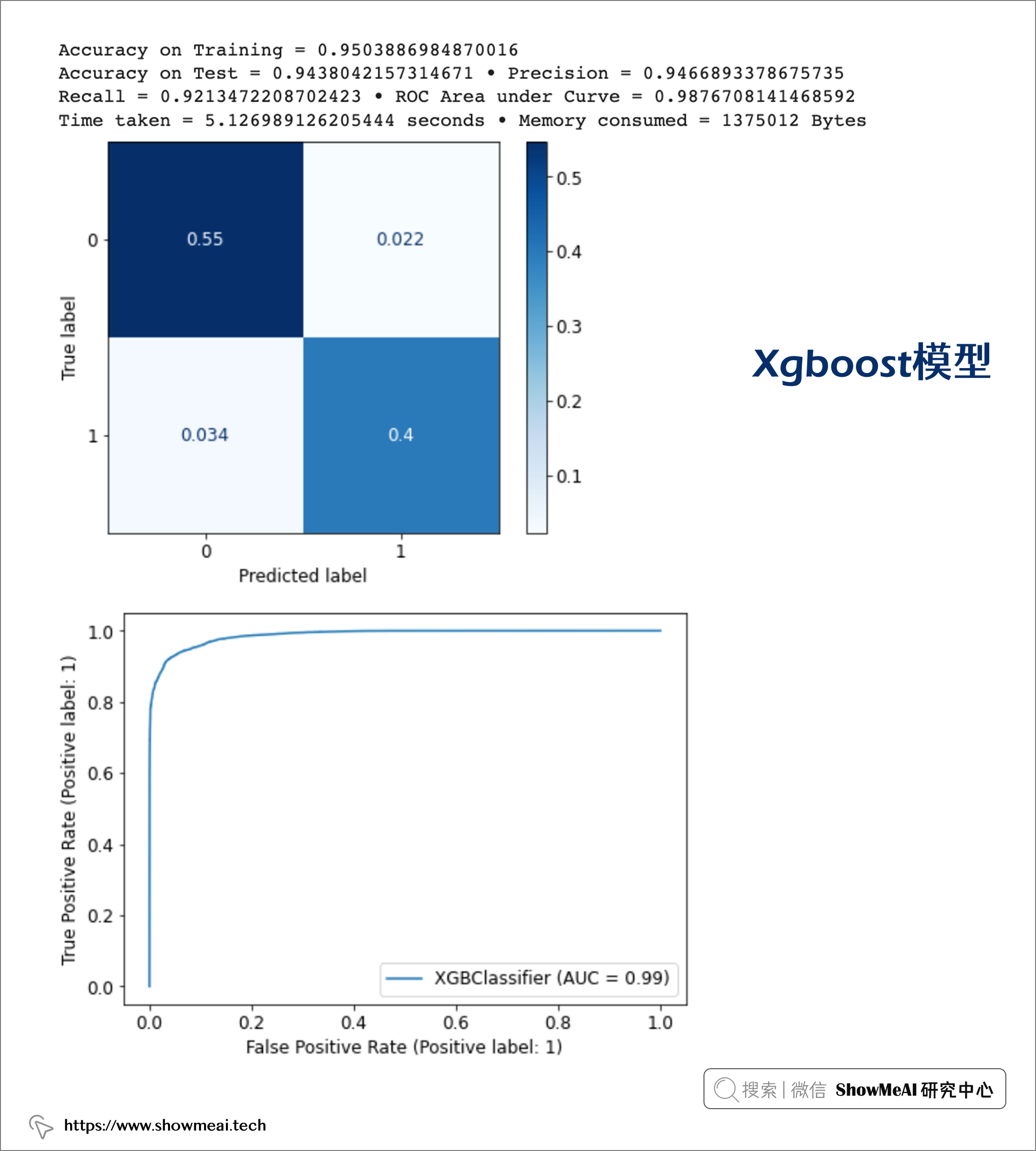
⑤ Xgboost模型
clf = XGBClassifier()

params = { 'max_depth': [3, 5, 6, 10, 15, 20],
           'learning_rate': [0.01, 0.1, 0.2, 0.3],
           'n_estimators': [100, 500, 1000]}

rscv = RandomizedSearchCV(estimator = clf,
                         param_distributions = params,
                         scoring = 'f1',
                         n_iter = 10,
                         verbose = 1)
rscv.fit(X_train, y_train)
rscv.predict(X_test)

# Parameter object to be passed through to function activation
params = rscv.best_params_

print("Best parameters:", params)
model_xgb = XGBClassifier(**params)

# Saving Output Metrics
model_xgb, accuracy_xgb, train_xgb, precision_xgb, recall_xgb, roc_xgb, tt_xgb, mu_xgb = get_model_metrics(model_xgb, X_train, X_test, y_train, y_test)
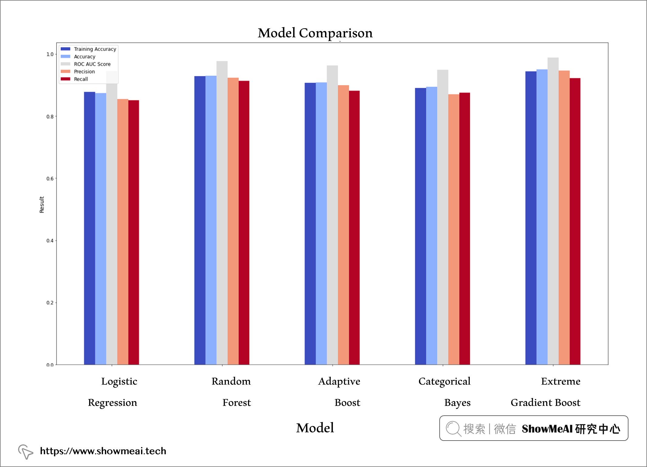
综合对比
如下我们对效果做一个综合对比,每个模型都应用了参数优化,在训练数据上的准确率不低于 88%,在测试数据上的准确率不低于 87%。
training_scores = [train_lr, train_rf, train_ada, train_cnb, train_xgb]
accuracy = [accuracy_lr, accuracy_rf, accuracy_ada, accuracy_cnb, accuracy_xgb]
roc_scores = [roc_lr, roc_rf, roc_ada, roc_cnb, roc_xgb]
precision = [precision_lr, precision_rf, precision_ada, precision_cnb, precision_xgb]
recall = [recall_lr, recall_rf, recall_ada, recall_cnb, recall_xgb]
time_scores = [tt_lr, tt_rf, tt_ada, tt_cnb, tt_xgb]
memory_scores = [mu_lr, mu_rf, mu_ada, mu_cnb, mu_xgb]

model_data = {'Model': ['Logistic Regression', 'Random Forest', 'Adaptive Boost',
                       'Categorical Bayes', 'Extreme Gradient Boost'],
            'Accuracy on Training' : training_scores,
            'Accuracy on Test' : accuracy,
            'ROC AUC Score' : roc_scores,
            'Precision' : precision,
            'Recall' : recall,
            'Time Elapsed (seconds)' : time_scores,
            'Memory Consumed (bytes)': memory_scores}

model_data = pd.DataFrame(model_data)
model_data

我们最终选择xgboost,它表现最好,在训练和测试中都表现出高性能,测试集上ROC-AUC值为 98,精度为 95,召回率为 92。
plt.rcParams["figure.figsize"] = (25,15)

ax1 = model_data.plot.bar(x = 'Model', y = ["Accuracy on Training", "Accuracy on Test", "ROC AUC Score",
                                            "Precision", "Recall"],
                          cmap = 'coolwarm')
ax1.legend()

ax1.set_title("Model Comparison", fontsize = 18)
ax1.set_xlabel('Model', fontsize = 14)
ax1.set_ylabel('Result', fontsize = 14, color = 'Black');
💡 模型可解释性
除了拿到最终性能良好的模型,在机器学习实际应用中,很重要的另外一件事情是结合业务场景进行解释,这能帮助业务后续提升。我们可以基于Xgboost自带的特征重要度和SHAP等完成这项任务。
对于SHAP工具库的使用介绍,欢迎大家阅读ShowMeAI的文章:
📘基于SHAP的机器学习可解释性实战
💦 XGBoost 特征重要性
from xgboost import plot_importance

model_xgb.get_booster().feature_names = ['type_of_travel', 'inflight_wifi_service', 'online_boarding',
       'seat_comfort', 'inflight_entertainment', 'on_board_service',
       'leg_room_service', 'cleanliness', 'class_business', 'class_eco']

plot_importance(model_xgb)
plt.show()
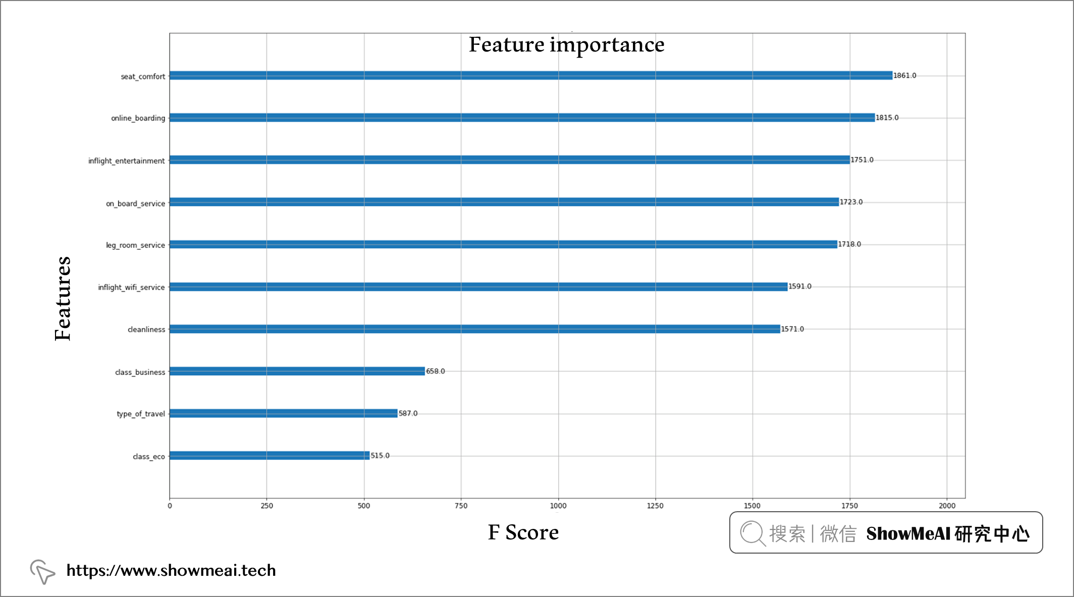
Xgboost给出的最重要的特征依次包括:座椅舒适度、在线登机、机上娱乐、机上服务质量、腿部空间、机上无线网络和清洁度。
💦 SHAP 模型和特征可解释性
为了分析模型在 SHAP 中的特征影响,首先使用 Python 的 pickle 库对模型进行 pickle。然后使用模型管道和我们选择的特征在 Shap 中创建了一个解释器,并将其应用于 X_train 数据集上。
import shap
# Saving test model.
pickle.dump(model_xgb, open('./Models/model_xgb.pkl', 'wb'))

explainer = shap.Explainer(model_xgb, feature_names = features)
shap_values = explainer(X_train)

shap.initjs()
shap.summary_plot(shap_values, X_train, class_names=model_xgb.classes_)
如果将平均 SHAP 值作为我们衡量特征重要性的指标,我们可以看到机上 Wi-Fi 服务是我们数据中最具影响力的特征,紧随其后的是旅行类型和在线登机。
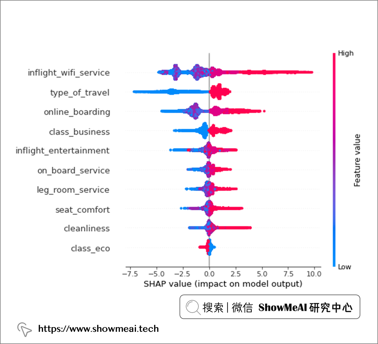
对于几乎每个特征,高取值(大部分是对这个特征维度的满意程度高)对预测有积极影响,而低特征值对预测有负面影响。机上 wi-fi 服务是我们数据集中最具影响力的特征,紧随其后的是旅行类型和在线登机流程。
💦 机上 Wi-Fi 服务 特征影响分析
shap.plots.scatter(shap_values[:, "inflight_wifi_service"], color=shap_values)

我们拿出最重要的特征『机上 Wi-Fi』进行进一步分析。上图中的横坐标为机上wifi满意度得分,纵坐标为SHAP值大小,颜色区分旅行类型(个人旅行编码为 0,商务旅行编码为 1)。
我们观察到:
-
个人旅行乘客:机上WiFi打分高对最终高满意度有更多的正面影响,而机上WiFi打分低对最终满意度低的贡献更大。
-
商务旅行乘客:无论他们的 Wi-Fi 服务体验如何,都有一部分是满意的(正 SHAP 值超过负值)。
💦 在线登机特征影响分析
shap.plots.scatter(shap_values[:, "online_boarding"], color=shap_values)
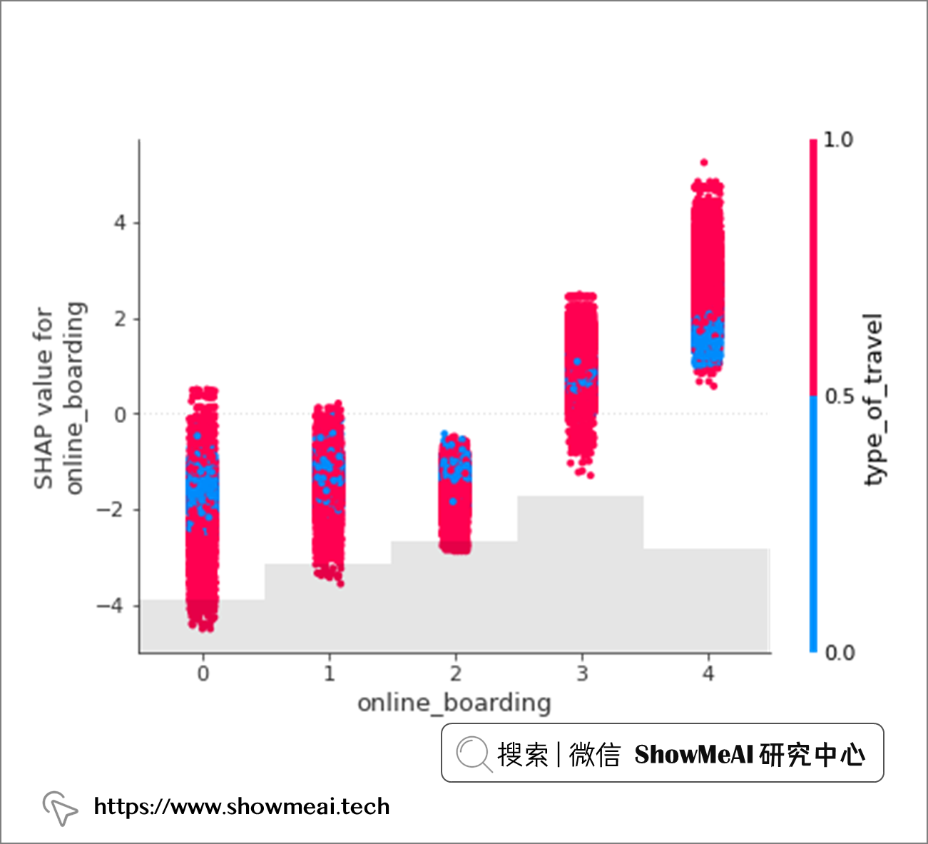
对『在线登机』特征的影响SHAP分析如上。无论是个人旅行还是商务出行,在线登机过程的低分都会对最终满意度输出产生负面影响。
💡 总结
在本篇内容中,我们结合航空出行场景,对航班乘客满意度进行了详尽的数据分析和建模预测,并进行了模型的可解释性分析。
我们效果最好的模型取得了95%的accuracy和0.987的auc得分,模型解释上可以看到影响满意度最重要的因素是机上 Wi-Fi 服务、在线登机、机上娱乐质量、餐饮、座椅舒适度、机舱清洁度和腿部空间。
参考资料
- 📘 航空公司乘客满意度数据集(Kaggle)
- 📘 美国航空公司的乘客不满意原因分析(CNN)
- 📘 新闻:随着飞机客满和票价上涨,旅客满意度下降(CNBC)
- 📘 数据分析实战:Python 数据分析实战教程:https://www.showmeai.tech/tutorials/40
- 📘 机器学习实战:手把手教你玩转机器学习系列:https://www.showmeai.tech/tutorials/41
- 📘 基于SHAP的机器学习可解释性实战:https://showmeai.tech/article-detail/337
- 📘 机器学习实战 | 机器学习特征工程最全解读:https://showmeai.tech/article-detail/208
推荐阅读
- 🌍 数据分析实战系列 :https://www.showmeai.tech/tutorials/40
- 🌍 机器学习数据分析实战系列:https://www.showmeai.tech/tutorials/41
- 🌍 深度学习数据分析实战系列:https://www.showmeai.tech/tutorials/42
- 🌍 TensorFlow数据分析实战系列:https://www.showmeai.tech/tutorials/43
- 🌍 PyTorch数据分析实战系列:https://www.showmeai.tech/tutorials/44
- 🌍 NLP实战数据分析实战系列:https://www.showmeai.tech/tutorials/45
- 🌍 CV实战数据分析实战系列:https://www.showmeai.tech/tutorials/46
- 🌍 AI 面试题库系列:https://www.showmeai.tech/tutorials/48


![[附源码]计算机毕业设计springboot体育馆场地预约管理系统](https://img-blog.csdnimg.cn/b63d789a3d6943c4a0b4e163a17acb98.png)