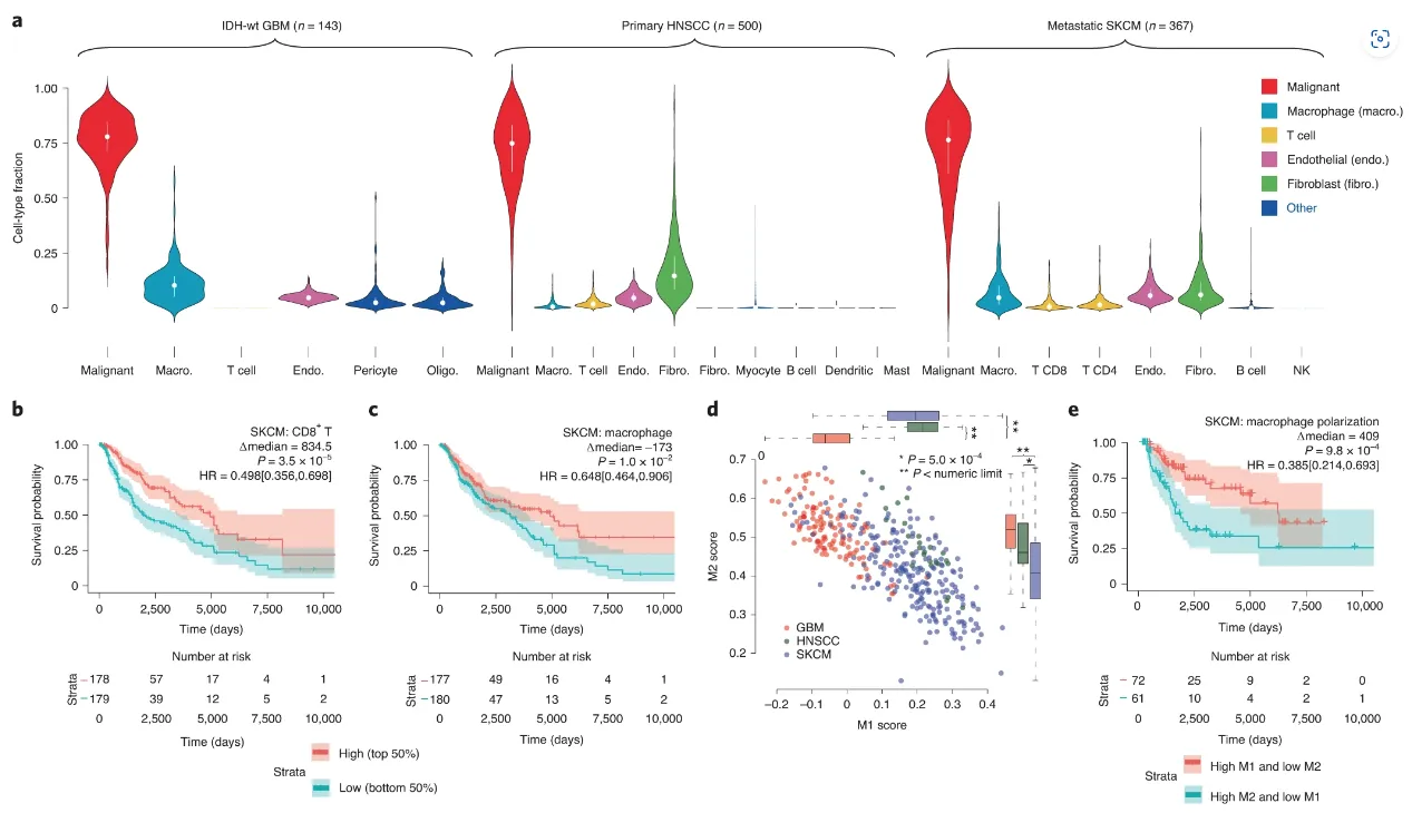
BayesPrism(贝叶斯棱镜法)可提取单细胞数据去卷积后将信息映射至bulkRNA数据

贝叶斯棱镜法作为一种工具可以根据scRNA数据(作为先验模型)去推断bulkRNA数据中肿瘤微环境组成(不同免疫细胞组分/不同细胞群)和基因表达情况。

开发者展示的图片就很形象了，左边图展示了把标注了不同细胞类型的单细胞数据作为先验信息(prior info)的基因信息和bulkRNA测序数据输入进贝叶斯棱镜算法，右图就是通过了棱镜算法之后慢慢地把bulkRNA测序数据中每个样本里所占的标注细胞类型的细胞百分比展示出来。

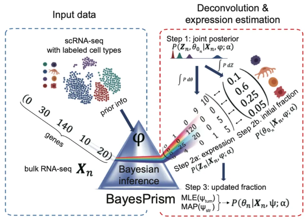
那么再通俗的来说，贝叶斯棱镜法就是将单细胞数据中的不同细胞亚群信息提取出来，并按照提取出来的信息将bulkRNA数据的每一个样本也分成不同细胞亚群(不够专业但方便理解)。

但其实类似的算法也有很多，另外一个比较热门的算法是CIBERSOTx，但相比于CIBERSOTx, 贝叶斯棱镜法利用了贝叶斯定理(Bayes’theorem)及吉布斯采样(Gibbs sampling)减少技术性批次效应和生物学差异。

从研究者发布的文章数据来看，贝叶斯棱镜法在估计实际细胞类型百分比得出的皮尔逊相关系数和误差均优于其他的算法。所以目前在选择算法时当然首选BayesPrism(贝叶斯棱镜法)~

最终分析结果部分会得到每个细胞亚群在样本中的百分比theta值、theta.cv值(theta值的变异信息), 不同细胞类型的特异基因的count矩阵值。

这跟之前写的Scissor算法有异曲同工之妙，一种是把bulkRNA数据的表型信息映射到单细胞数据上去，贝叶斯棱镜法是把单细胞数据的表型信息映射到bulkRNA数据上(不够专业但方便理解)。

Scissor算法：https://mp.weixin.qq.com/s/yUaeJKpuF1NzaD0fnhhUuQ

分析步骤-from github

1、加载BayesPrism R包

library("devtools");
install_github("Danko-Lab/BayesPrism/BayesPrism")
suppressWarnings(library(BayesPrism))
#> Loading required package: snowfall
#> Loading required package: snow
#> Loading required package: NMF
#> Loading required package: pkgmaker
#> Loading required package: registry
#> Loading required package: rngtools
#> Loading required package: cluster
#> NMF - BioConductor layer [OK] | Shared memory capabilities [NO: bigmemory] | Cores 71/72
#>   To enable shared memory capabilities, try: install.extras('
#> NMF
#> ')

2、加载示例数据

load("../tutorial.dat/tutorial.gbm.rdata")
ls()
#> [1] "bk.dat"            "cell.state.labels" "cell.type.labels"  "sc.dat"

sc.dat: 单细胞数据

cell.state.labels: 细胞状态标签

cell.type.labels: 细胞类型标签

bk.dat: bulk RNA数据

dim(bk.dat)
#> [1]   169 60483
head(rownames(bk.dat))
#> [1] "TCGA-06-2563-01A-01R-1849-01" "TCGA-06-0749-01A-01R-1849-01" "TCGA-06-5418-01A-01R-1849-01" "TCGA-06-0211-01B-01R-1849-01" "TCGA-19-2625-01A-01R-1850-01" "TCGA-19-4065-02A-11R-2005-01"
head(colnames(bk.dat))
#> [1] "ENSG00000000003.13" "ENSG00000000005.5"  "ENSG00000000419.11" "ENSG00000000457.12" "ENSG00000000460.15" "ENSG00000000938.11"

dim(sc.dat)
#> [1] 23793 60294
head(rownames(sc.dat))
#> [1] "PJ016.V3" "PJ016.V4" "PJ016.V5" "PJ016.V6" "PJ016.V7" "PJ016.V8"
head(colnames(sc.dat))

bulk RNA 和 scRNA 数据格式均行是样本名，基因是列名。

bulk RNA和scRNA 要采用一样的基因信息，代码块中均为ensembl ID。

此外，bulkRNA数据需采用count数据。若count数据不可用时，TPM，RPM，RPKM，FPKM等也是可接受的，但不要进行log转换。

sort(table(cell.type.labels))
#> cell.type.labels
#>       tcell       oligo    pericyte endothelial     myeloid       tumor 
#>          67         160         489         492        2505       20080

sort(table(cell.state.labels))
#> cell.state.labels
#> PJ017-tumor-6 PJ032-tumor-5     myeloid_8 PJ032-tumor-4 PJ032-tumor-3 PJ017-tumor-5         tcell PJ032-tumor-2 PJ030-tumor-5     myeloid_7 PJ035-tumor-8 PJ017-tumor-4 PJ017-tumor-3 PJ017-tumor-2 PJ017-tumor-0 PJ017-tumor-1 PJ018-tumor-5     myeloid_6     myeloid_5 PJ035-tumor-7         oligo PJ048-tumor-8 PJ032-tumor-1 PJ032-tumor-0 PJ048-tumor-7 PJ025-tumor-9 PJ035-tumor-6 PJ048-tumor-6 PJ016-tumor-6 PJ018-tumor-4     myeloid_4 PJ048-tumor-5 PJ048-tumor-4 PJ016-tumor-5 PJ025-tumor-8 PJ048-tumor-3 PJ035-tumor-5 PJ030-tumor-4 PJ018-tumor-3 PJ016-tumor-4 PJ025-tumor-7     myeloid_3 PJ035-tumor-4     myeloid_2 PJ025-tumor-6 PJ018-tumor-2 PJ030-tumor-3 PJ016-tumor-3 PJ025-tumor-5 PJ030-tumor-2 PJ018-tumor-1 PJ035-tumor-3 PJ048-tumor-2 PJ018-tumor-0 PJ048-tumor-1 PJ035-tumor-2 PJ035-tumor-1 PJ016-tumor-2 PJ030-tumor-1      pericyte   endothelial PJ035-tumor-0 PJ025-tumor-4     myeloid_1 PJ048-tumor-0     myeloid_0 PJ030-tumor-0 PJ025-tumor-3 PJ016-tumor-1 PJ016-tumor-0 PJ025-tumor-2 PJ025-tumor-1 PJ025-tumor-0 
#>            22            41            49            57            62            64            67            72            73            75            81            83            89           101           107           107           113           130           141           150           160           169           171           195           228           236           241           244           261           262           266           277           303           308           319           333           334           348           361           375           381           382           385           386           397           403           419           420           421           425           429           435           437           444           463           471           474           481           482           489           492           512           523           526           545           550           563           601           619           621           630           941           971

cell.type.labels代表着纳入分析的scRNA数据中不同细胞类型的数量。

如何进行cell type分类，开发团队提供的依据/建议是：Define cell types as the cluster of cells having a sufficient number of significantly differentially expressed genes than other cell types, e.g., greater than 50 or even 100.

简单来说就是划分出来的不同细胞类型是存在着显著的表观等差别的。

sort(table(cell.state.labels))
#> cell.state.labels
#> PJ017-tumor-6 PJ032-tumor-5     myeloid_8 PJ032-tumor-4 PJ032-tumor-3 PJ017-tumor-5         tcell PJ032-tumor-2 PJ030-tumor-5     myeloid_7 PJ035-tumor-8 PJ017-tumor-4 PJ017-tumor-3 PJ017-tumor-2 PJ017-tumor-0 PJ017-tumor-1 PJ018-tumor-5     myeloid_6     myeloid_5 PJ035-tumor-7         oligo PJ048-tumor-8 PJ032-tumor-1 PJ032-tumor-0 PJ048-tumor-7 PJ025-tumor-9 PJ035-tumor-6 PJ048-tumor-6 PJ016-tumor-6 PJ018-tumor-4     myeloid_4 PJ048-tumor-5 PJ048-tumor-4 PJ016-tumor-5 PJ025-tumor-8 PJ048-tumor-3 PJ035-tumor-5 PJ030-tumor-4 PJ018-tumor-3 PJ016-tumor-4 PJ025-tumor-7     myeloid_3 PJ035-tumor-4     myeloid_2 PJ025-tumor-6 PJ018-tumor-2 PJ030-tumor-3 PJ016-tumor-3 PJ025-tumor-5 PJ030-tumor-2 PJ018-tumor-1 PJ035-tumor-3 PJ048-tumor-2 PJ018-tumor-0 PJ048-tumor-1 PJ035-tumor-2 PJ035-tumor-1 PJ016-tumor-2 PJ030-tumor-1      pericyte   endothelial PJ035-tumor-0 PJ025-tumor-4     myeloid_1 PJ048-tumor-0     myeloid_0 PJ030-tumor-0 PJ025-tumor-3 PJ016-tumor-1 PJ016-tumor-0 PJ025-tumor-2 PJ025-tumor-1 PJ025-tumor-0 
#>            22            41            49            57            62            64            67            72            73            75            81            83            89           101           107           107           113           130           141           150           160           169           171           195           228           236           241           244           261           262           266           277           303           308           319           333           334           348           361           375           381           382           385           386           397           403           419           420           421           425           429           435           437           444           463           471           474           481           482           489           492           512           523           526           545           550           563           601           619           621           630           941           971

cell.state.labels代表着纳入分析的scRNA数据中不同细胞类型的细分状态。

开发者给出的例子中对tumor和myeloid细胞进行了细分，原因是开发团队觉得肿瘤和髓系细胞中内部的不同细胞亚型具有不同的生物学作用而且很重要。

对于使用者而言，选择什么细胞进行细分“state”亚群这就根据自身的研究而定。若不想细分也可以，后续可以把相关参数设置NULL。

细分后定义的细胞状态亚群群的细胞数量至少需要>20，严格一点需要>50.

如何进行cell state分类，开发团队提供的依据/建议是：For clusters that are too similar in transcription, we recommend treating them as cell states, which will be summed up before the final Gibbs sampling. Therefore, cell states are often suitable for cells that form a continuum on the phenotypic manifold rather than distinct clusters.

简单来说就是对于转录特征很相似的细胞簇(表观上很相似)，但可能在功能上/生物学意义上存在一定的差别，建议设置不同的细胞状态，比如肿瘤细胞存在很强的异质性/很有探究价值等。

3、对细胞类型和细胞状态进行质量控制

plot.cor.phi (input=sc.dat,
                         input.labels=cell.state.labels,
                         title="cell state correlation",
                         #specify pdf.prefix if need to output to pdf
                         #pdf.prefix="gbm.cor.cs", 
                         cexRow=0.2, cexCol=0.2,
                         margins=c(2,2)
                         )

plot.cor.phi (input=sc.dat, 
                         input.labels=cell.type.labels, 
                         title="cell type correlation",
                         #specify pdf.prefix if need to output to pdf
                         #pdf.prefix="gbm.cor.ct",
                         cexRow=0.5, cexCol=0.5,
                         )

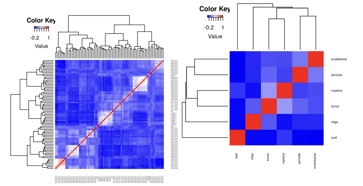
分别对细胞类型和细胞状态进行相关性分析，这个步骤是识别相似的簇，若观察到相似的簇，应考虑合并。

4、可视化scRNA数据中的异常基因

sc.stat <- plot.scRNA.outlier(
  input=sc.dat, #make sure the colnames are gene symbol or ENSMEBL ID 
  cell.type.labels=cell.type.labels,
  species="hs", #currently only human(hs) and mouse(mm) annotations are supported
  return.raw=TRUE #return the data used for plotting. 
  #pdf.prefix="gbm.sc.stat" specify pdf.prefix if need to output to pdf
)
#> EMSEMBLE IDs detected.

有很多大量表达基因，比如核糖体蛋白质基因和线粒体基因，它们在分簇的时候往往给不了有用的信息，还会干扰分簇并使结果产生偏倚，因此需要去除。

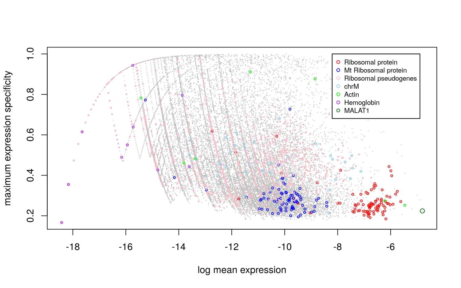
如图所示：核糖体蛋白质基因通常表现出高平均表达(X轴)和低细胞类型特异性得分(Y轴)。

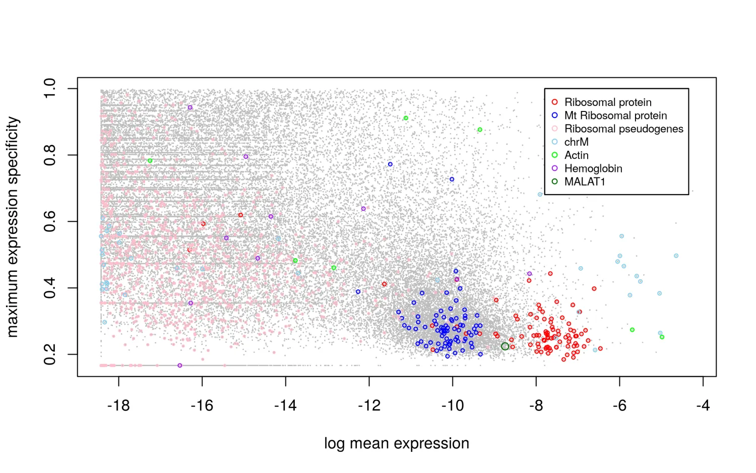
5、可视化bulkRNA数据中的异常基因

bk.stat <- plot.bulk.outlier(
  bulk.input=bk.dat,#make sure the colnames are gene symbol or ENSMEBL ID 
    sc.input=sc.dat, #make sure the colnames are gene symbol or ENSMEBL ID 
  cell.type.labels=cell.type.labels,
  species="hs", #currently only human(hs) and mouse(mm) annotations are supported
  return.raw=TRUE
  #pdf.prefix="gbm.bk.stat" specify pdf.prefix if need to output to pdf
)
#> EMSEMBLE IDs detected.

6、过滤scRNA数据的异常基因

sc.dat.filtered <- cleanup.genes (input=sc.dat,
                                  input.type="count.matrix",
                                  species="hs", 
                                  gene.group=c( "Rb","Mrp","other_Rb","chrM","MALAT1","chrX","chrY") ,
                                  exp.cells=5)
#> EMSEMBLE IDs detected.
#> number of genes filtered in each category: 
#>       Rb      Mrp other_Rb     chrM   MALAT1     chrX     chrY 
#>       89       78     1011       37        1     2464      594 
#> A total of  4214  genes from Rb Mrp other_Rb chrM MALAT1 chrX chrY  have been excluded 
#> A total of  24343  gene expressed in fewer than  5  cells have been excluded

去除设置的细胞群基因。

7、检查基因与不同基因集之间的相关性

#note this function only works for human data. For other species, you are advised to make plots by yourself.
plot.bulk.vs.sc (sc.input = sc.dat.filtered,
                            bulk.input = bk.dat
                            #pdf.prefix="gbm.bk.vs.sc" specify pdf.prefix if need to output to pdf
)
#> EMSEMBLE IDs detected.

8、提取蛋白编码基因

sc.dat.filtered.pc <-  select.gene.type (sc.dat.filtered,
                                        gene.type = "protein_coding")
#> EMSEMBLE IDs detected.
#> number of genes retained in each category: 
#> 
#> protein_coding 
#>          16148

9、构建BayesPrism模型

myPrism <- new.prism(
  reference=sc.dat.filtered.pc, 
  mixture=bk.dat,
  input.type="count.matrix", 
  cell.type.labels = cell.type.labels, 
  cell.state.labels = cell.state.labels,
  key="tumor", 
  outlier.cut=0.01,
  outlier.fraction=0.1,
)
#> number of cells in each cell state 
#> cell.state.labels
#> PJ017-tumor-6 PJ032-tumor-5     myeloid_8 PJ032-tumor-4 PJ032-tumor-3 PJ017-tumor-5         tcell PJ032-tumor-2 PJ030-tumor-5     myeloid_7 PJ035-tumor-8 PJ017-tumor-4 PJ017-tumor-3 PJ017-tumor-2 PJ017-tumor-0 PJ017-tumor-1 PJ018-tumor-5     myeloid_6     myeloid_5 PJ035-tumor-7         oligo PJ048-tumor-8 PJ032-tumor-1 PJ032-tumor-0 PJ048-tumor-7 PJ025-tumor-9 PJ035-tumor-6 PJ048-tumor-6 PJ016-tumor-6 PJ018-tumor-4     myeloid_4 PJ048-tumor-5 PJ048-tumor-4 PJ016-tumor-5 PJ025-tumor-8 PJ048-tumor-3 PJ035-tumor-5 PJ030-tumor-4 PJ018-tumor-3 PJ016-tumor-4 PJ025-tumor-7     myeloid_3 PJ035-tumor-4     myeloid_2 PJ025-tumor-6 PJ018-tumor-2 PJ030-tumor-3 PJ016-tumor-3 PJ025-tumor-5 PJ030-tumor-2 PJ018-tumor-1 PJ035-tumor-3 PJ048-tumor-2 PJ018-tumor-0 PJ048-tumor-1 PJ035-tumor-2 PJ035-tumor-1 PJ016-tumor-2 PJ030-tumor-1      pericyte   endothelial PJ035-tumor-0 PJ025-tumor-4     myeloid_1 PJ048-tumor-0     myeloid_0 PJ030-tumor-0 PJ025-tumor-3 PJ016-tumor-1 PJ016-tumor-0 PJ025-tumor-2 PJ025-tumor-1 PJ025-tumor-0 
#>            22            41            49            57            62            64            67            72            73            75            81            83            89           101           107           107           113           130           141           150           160           169           171           195           228           236           241           244           261           262           266           277           303           308           319           333           334           348           361           375           381           382           385           386           397           403           419           420           421           425           429           435           437           444           463           471           474           481           482           489           492           512           523           526           545           550           563           601           619           621           630           941           971 
#> Number of outlier genes filtered from mixture = 6 
#> Aligning reference and mixture... 
#> Nornalizing reference...

#Note that outlier.cut and outlier.fraction=0.1 filter genes in X whose expression fraction is greater than outlier.cut (Default=0.01) in more than outlier.fraction (Default=0.1) of bulk data. 
#Typically for dataset with reasonable quality control, very few genes will be filtered. 
#Removal of outlier genes will ensure that the inference will not be dominated by outliers, which sometimes may be resulted from poor QC in mapping.

input.type 除了常规的设置"count.matrix"以外，还有另一种设置类型是“GEP”，开发者给出的解释是：the other option for input.type is "GEP" (gene expression profile) which is a cell state by gene matrix. This option is used when using reference derived from other assays, such as sorted bulk data. 这个GEP暂时没有理解，求高手指点~

参数key是cell.type.label 中对应于使用者自行命名的恶性细胞的名称，比如在cell.type.label中命名为tumor，那么key参数后面也可以写tumor。如果没有恶性细胞，也可以设置为NULL，在这种情况下，所有类型的细胞将被会被算法平等对待。

10、运行BayesPrism模型

bp.res <- run.prism(prism = myPrism, n.cores=50)

如果电脑配置比较弱，建议把n.cores降低一点。笔者就对自己的电脑过于自信而不降低n.cores值，导致运行这个算法的时候电脑被干死机过...

11、提取细胞比例theta值

# extract posterior mean of cell type fraction theta
theta <- get.fraction (bp=bp.res,
            which.theta="final",
            state.or.type="type")

head(theta)
#>                                  tumor    myeloid     pericyte endothelial        tcell        oligo
#> TCGA-06-2563-01A-01R-1849-01 0.8392297 0.04329259 2.999022e-02  0.07528272 6.474488e-04 0.0115573149
#> TCGA-06-0749-01A-01R-1849-01 0.7090654 0.17001073 8.995526e-07  0.01275526 1.179331e-06 0.1081665709
#> TCGA-06-5418-01A-01R-1849-01 0.8625322 0.09839143 9.729268e-03  0.02416954 7.039913e-07 0.0051768589
#> TCGA-06-0211-01B-01R-1849-01 0.8893449 0.04482991 1.131622e-02  0.05435490 2.508238e-06 0.0001515524
#> TCGA-19-2625-01A-01R-1850-01 0.9406438 0.03546026 1.932740e-03  0.01309753 4.535897e-06 0.0088610997
#> TCGA-19-4065-02A-11R-2005-01 0.6763166 0.08374439 1.849921e-01  0.01918132 3.541126e-04 0.0354114398

这一步就是提取每种细胞亚群占每一个样本的比例。可以自行计算，同一个样本的不同细胞类型之和为1。

12、提取细胞比例theta值的变异分数

# extract coefficient of variation (CV) of cell type fraction
theta.cv <- bp.res@posterior.theta_f@theta.cv

head(theta.cv)
#>                                     tumor      myeloid     pericyte endothelial      tcell       oligo
#> TCGA-06-2563-01A-01R-1849-01 0.0001722829 0.0016025331 0.0026568433 0.001853843 0.05452368 0.005606057
#> TCGA-06-0749-01A-01R-1849-01 0.0002333853 0.0006859332 0.8109050326 0.005683516 0.74729658 0.001276784
#> TCGA-06-5418-01A-01R-1849-01 0.0001601128 0.0009389782 0.0070872942 0.004131925 0.83670176 0.011362855
#> TCGA-06-0211-01B-01R-1849-01 0.0001175529 0.0014412303 0.0055064706 0.001673105 0.60905434 0.280609474
#> TCGA-19-2625-01A-01R-1850-01 0.0001327408 0.0023661566 0.0335184780 0.006286823 0.73453327 0.006138184
#> TCGA-19-4065-02A-11R-2005-01 0.0002862600 0.0012227981 0.0009100677 0.005660069 0.06371147 0.002243368

这里的变异系数(CV)反应了后验分布的变异程度，theta值越高CV值就越低。

在执行排名相关的统计分析时，例如斯皮尔曼等级相关系数，研究者可以选择在变异系数低于某个阈值（例如小于0.1）的情况下将 theta 设置为零(更高的排序)。这种做法可以帮助屏蔽那些在后验分布中变异性较小、较为确定的测量值，以便更清晰地聚焦于那些变异性更高的数据点。

13、提取特定细胞类型基因count矩阵的后验平均值

# extract posterior mean of cell type-specific gene expression count matrix Z  
Z.tumor <- get.exp (bp=bp.res,
                          state.or.type="type",
                          cell.name="tumor")

head(t(Z.tumor[1:5,]))
#>                    TCGA-06-2563-01A-01R-1849-01 TCGA-06-0749-01A-01R-1849-01 TCGA-06-5418-01A-01R-1849-01 TCGA-06-0211-01B-01R-1849-01 TCGA-19-2625-01A-01R-1850-01
#> ENSG00000130876.10                       55.980                      444.980                        9.000                       56.996                       15.996
#> ENSG00000165244.6                       206.344                       38.096                      291.872                      530.732                      507.788
#> ENSG00000173597.7                        17.100                        6.588                       21.804                       28.744                       10.800
#> ENSG00000158022.6                         0.000                        0.476                        2.616                        0.960                        7.824
#> ENSG00000167220.10                     2273.824                     1060.976                     2775.180                     2368.016                     2084.620
#> ENSG00000126106.12                      678.468                      685.948                      481.000                      698.888                     1296.080

14、保存数据

#save the result
save(bp.res, file="bp.res.rdata")

后续就可以根据不同细胞比例的theta值，CV值，或者特意基因数据进行不同细胞比率的图形绘制，或者跟生存数据联合分析等

除了上述的个性化分析以外，开发者内置了基于BayesPrism的恶性细胞表达嵌入学习模块(对恶性细胞进行非负矩阵分解分簇)

这块内容在分析前需对BayesPrism模型设置参数key！

15、提取信息

Z.tum.norm <- t(bp.res@reference.update@psi)
estim.Z.tum.norm <- nmf(Z.tum.norm, rank=2:12, seed=123456)
plot(estim.Z.tum.norm)
consensusmap(estim.Z.tum.norm, labCol=NA, labRow=NA)

16、运行NMF

ebd.res <- learn.embedding.nmf (bp = bp.res, 
                                #bp.res needs to be run under the tumor mode.
                                K = 2,
                                cycle = 20, #EM typically converges in 50 cycles. set to 20 for demo
                                compute.elbo = T)
str(ebd.res)
#> List of 4
#> $ eta_prior: num [1:5, 1:16145] 6.91e-07 2.16e-06 1.72e-05 4.24e-07 2.61e-06 ...
 #>   ..- attr(*, "dimnames")=List of 2
 #>   .. ..$ : chr [1:5] "program-1" "program-2" "program-3" "program-4" ...
 #>   .. ..$ : chr [1:16145] "ENSG00000130876.10" "ENSG00000165244.6" "ENSG00000173597.7" "ENSG00000158022.6" ...
 #>  $ eta_post : num [1:5, 1:16145] 7.88e-07 2.37e-06 1.34e-05 1.11e-07 1.67e-06 ...
 #>   ..- attr(*, "dimnames")=List of 2
 #>   .. ..$ : chr [1:5] "program-1" "program-2" "program-3" "program-4" ...
 #>   .. ..$ : chr [1:16145] "ENSG00000130876.10" "ENSG00000165244.6" "ENSG00000173597.7" "ENSG00000158022.6" ...
 #>  $ omega    : num [1:169, 1:5] 0.701906 0.000555 0.324483 0.627062 0.172039 ...
 #>   ..- attr(*, "dimnames")=List of 2
 #>   .. ..$ : chr [1:169] "TCGA-06-2563-01A-01R-1849-01" "TCGA-06-0749-01A-01R-1849-01" "TCGA-06-5418-01A-01R-1849-01" "TCGA-06-0211-01B-01R-184
 #>   .. ..$ : chr [1:5] "program-1" "program-2" "program-3" "program-4" ...
 #>  $ elbo     : num [1:21] Inf 1.06e+11 1.06e+11 1.06e+11 1.06e+11 ...

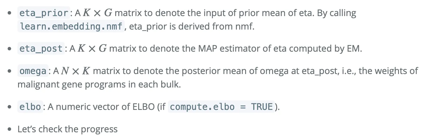
大概的对应解释是：

● eta_prior（先验均值矩阵）：这是一个 K × G 的矩阵，用来表示 eta 的先验均值输入。在调用 learn.embedding.nmf 函数时，可以从非负矩阵分解（NMF）得到 eta_prior。简单来说，这个矩阵包含了在开始模型估计之前，我们对每个基因表达程序的预期水平的先验知识。

● eta_post（后验估计矩阵）：这也是一个 K × G 的矩阵，表示通过期望最大化（EM）算法计算得到的 eta 的最大后验（MAP）估计值。这个矩阵更新了我们对每个基因表达程序强度的估计，基于实际观测数据进行调整。

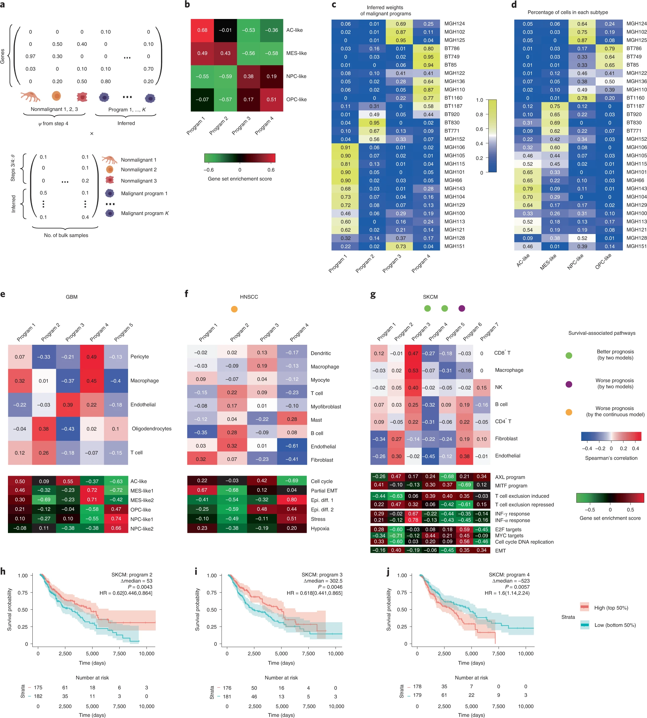
● omega（后验均值矩阵）：这是一个 N × K 的矩阵，用于表示在 eta_post（即 eta 的后验估计值）下 omega 的后验均值，也就是每个批量样本中恶性基因程序的权重。这个矩阵反映了在具体样本中，不同恶性基因表达程序的相对表达强度。

● elbo（证据下界向量）：如果设置 compute.elbo = TRUE，则这是一个数值向量，表示每次迭代计算的证据下界（ELBO）。ELBO是一个在统计模型中用来衡量模型拟合优度的指标，通常用于贝叶斯框架中评估模型的表现。

得到了不同簇的数据之后，后续还可以进行富集分析观察每个簇中的通路情况~

参考资料：

1、https://www.bayesprism.org/pages/tutorial_deconvolution (网站上还可以对数据进行在线分析哦~）

2、https://github.com/Danko-Lab/BayesPrism/tree/main (github)

3、Cell type and gene expression deconvolution with BayesPrism enables Bayesian integrative analysis across bulk and single-cell RNA sequencing in oncology. Nat Cancer. 2022 Apr;3(4):505-517.

4、生信技能树推文： https://mp.weixin.qq.com/s/swPDu2PoGTBEutzaR7YYSg https://mp.weixin.qq.com/s/3dZQxDdY6M1WwMMcus5Gkg

致谢：感谢曾老师，小洁老师以及生信技能树团队全体成员。

注：若对内容有疑惑或者有发现明确错误的朋友，请联系后台(欢迎交流)。更多内容可关注公众号：生信方舟

- END -