欢迎大家关注全网生信学习者系列:
- WX公zhong号:生信学习者
- Xiao hong书:生信学习者
- 知hu:生信学习者
- CDSN:生信学习者2
介绍
微生物的物种差异分析是一项关键的生物信息学任务,旨在识别不同生物群落或样本组之间在物种组成上的差异。这种分析对于理解微生物群落的结构、功能以及它们在不同环境或宿主状态下的作用至关重要。考虑到微生物数据的特定特点,例如稀疏性、样本间抽样分数的差异等,传统的统计方法可能不足以准确揭示组间的微生物差异。
ANCOMBC-2(Analysis of Compositions of Microbiomes with Bias Correction 2)算法是针对这些挑战而设计的,它提供了一种有效的方法来识别微生物组数据中的组间标记物。
加载R包
library(readr)
library(openxlsx)
library(tidyverse)
library(ggpubr)
library(ANCOMBC)
library(SingleCellExperiment)
library(DT)
library(phyloseq)
# BiocManager::install("microbiome")
library(microbiome)
# BiocManager::install("mia")
library(mia)
导入数据
大家通过以下链接下载数据:
- 百度网盘链接:https://pan.baidu.com/s/1fz5tWy4mpJ7nd6C260abtg
- 提取码: 请关注WX公zhong号_生信学习者_后台发送 复现gmsb 获取提取码
# OTU table
otu_table <- read_tsv("./data/GMSB-data/otu-table.tsv")

# Taxonomy table
tax <- read_tsv("./data/GMSB-data/taxonomy.tsv")

# Metadata
meta_data <- read_csv("./data/GMSB-data/df_v1.csv")
数据预处理
-
Data cleaning:数据清洗
-
Phyloseq object:生成phyloseq数据对象
-
aggregate_taxa:累加genus/species丰度
-
TreeSummarizedExperiment:生成TreeSummarizedExperiment数据对象
# Data cleaning
## Generate a combined OTU/taxonomy table
combined_table <- otu_table %>%
  dplyr::left_join(
    tax %>%
      dplyr::select(`Feature ID`, Taxon),
    by = join_by(`#OTU ID` == `Feature ID`)
  )

## Clean the otu table
otu_id <- otu_table$`#OTU ID`
otu_table <- data.frame(otu_table[, -1], check.names = FALSE, row.names = otu_id)

## Clean the taxonomy table
otu_id <- tax$`Feature ID`
tax <- data.frame(tax[, - c(1, 3)], row.names = otu_id)
tax <- tax %>%
  tidyr::separate(col = Taxon,
           into = c("Kingdom", "Phylum", "Class", "Order",
                    "Family", "Genus", "Species"),
           sep = ";") %>%
  dplyr::rowwise() %>%
  dplyr::mutate_all(function(x) strsplit(x, "__")[[1]][2]) %>%
  dplyr::mutate(Species = ifelse(!is.na(Species) & !is.na(Genus),
                          paste(ifelse(strsplit(Genus, "")[[1]][1] == "[",
                                       strsplit(Genus, "")[[1]][2],
                                       strsplit(Genus, "")[[1]][1]), Species, sep = "."),
                          NA)) %>%
  dplyr::ungroup()
tax <- as.matrix(tax)
rownames(tax) <- otu_id
tax[tax == ""] <- NA

## Clean the metadata
meta_data$status <- factor(meta_data$status, levels = c("nc", "sc"))
meta_data$time2aids <- factor(meta_data$time2aids,
                             levels = c("never", "> 10 yrs",
                                        "5 - 10 yrs", "< 5 yrs"))

# Phyloseq object
OTU <- phyloseq::otu_table(otu_table, taxa_are_rows = TRUE)
META <- phyloseq::sample_data(meta_data)
phyloseq::sample_names(META) <- meta_data$sampleid
TAX <- phyloseq::tax_table(tax)
otu_data <- phyloseq::phyloseq(OTU, TAX, META)
otu_data <- phyloseq::subset_samples(otu_data, group1 != "missing")

# aggregate_taxa abundance
genus_data <- microbiome::aggregate_taxa(otu_data, "Genus")
species_data <- microbiome::aggregate_taxa(otu_data, "Species")

# TreeSummarizedExperiment object
tse <- mia::makeTreeSummarizedExperimentFromPhyloseq(otu_data)

tse
class: TreeSummarizedExperiment
dim: 6111 241
metadata(0):
assays(1): counts
rownames(6111): 000e1601e0051888d502cd6a535ecdda 0011d81f43ec49d21f2ab956ab12de2f ...
  fff3a05f150a52a2b6c238d2926a660d fffc6ea80dc6bb8cafacbab2d3b157b3
rowData names(7): Kingdom Phylum ... Genus Species
colnames(241): F-163 F-165 ... F-382 F-383
colData names(45): sampleid subjid ... hbv hcv
reducedDimNames(0):
mainExpName: NULL
altExpNames(0):
rowLinks: NULL
rowTree: NULL
colLinks: NULL
colTree: NULL
Primary group at species level
-
Number of stool samples
241, -
Number of taxa
128.
使用 ANCOMBC-2算法对Primary group分组间微生物species水平进行差异分析。ANCOMBC-2(Analysis of Compositions of Microbiomes with Bias Correction 2)是一种用于微生物组数据差异丰度分析的方法。它的核心原理是估计未知的抽样分数并纠正由样本间抽样分数的差异引起的偏差。以下是关于ANCOMBC-2算法原理的详细解释:
- 抽样分数的概念:抽样分数定义为一个随机样本中分类单元的预期绝对丰度与其在生态系统单位体积样本来源中的绝对丰度的比率。由于不同样本可能有不同的抽样分数,这会导致观察到的计数在样本间不可比。
- 绝对丰度和相对丰度:绝对丰度数据使用线性回归框架建模,而相对丰度的变化会影响所有物种的相对丰度。ANCOMBC-2方法考虑到了这一点,并在分析中进行了适当的处理。
- 偏差校正:ANCOMBC-2算法估计并校正由样本间抽样分数差异引起的偏差。这包括样本库大小的标准化和微生物载量的差异考虑。
- 统计检验:ANCOMBC-2提供具有适当p值的统计有效检验,为每个分类单元的差异丰度提供置信区间,并控制错误发现速率(FDR),同时保持足够的统计检验力。
- 算法实现:ANCOMBC-2在计算上易于实现,并且可以应用于跨截面和重复测量数据。它支持两组比较、连续协变量测试和多组比较,包括全局检验、成对方向检验、Dunnett类型检验和趋势检验。
- 数据输入和输出:ANCOMBC-2需要输入数据集和相应的模型公式,输出包括log fold changes、标准误差、W统计量、p值和调整后的p值等,以及是否通过敏感性分析的标志。
- 结构零的处理:ANCOMBC-2可以识别和处理结构零,即在某些组中完全或几乎完全缺失的计数。这有助于更准确地识别差异丰度的分类单元。
if (file.exists("./data/GMSB-data/rds/primary_ancombc2_species.rds")) {
  primary_ancombc2_species_output <- readRDS("./data/GMSB-data/rds/primary_ancombc2_species.rds")
} else {
primary_ancombc2_species_output <- ancombc2(
  data = tse,
  assay_name = "counts",
  tax_level = "Species",
  fix_formula = "group1 + abx_use",
  rand_formula = NULL,
  p_adj_method = "BY",
  prv_cut = 0.10,
  lib_cut = 1000,
  s0_perc = 0.05,
  group = "group1",
  struc_zero = TRUE,
  neg_lb = TRUE,
  alpha = 0.05,
  n_cl = 8,
  verbose = TRUE,
  global = TRUE,
  pairwise = TRUE,
  dunnet = TRUE,
  trend = TRUE,
  iter_control = list(tol = 1e-2, max_iter = 20, verbose = TRUE),
  em_control = list(tol = 1e-5, max_iter = 100),
  lme_control = lme4::lmerControl(),
  mdfdr_control = list(fwer_ctrl_method = "holm", B = 100),
  trend_control = list(contrast = list(matrix(c(1, 0, 0,
                                                -1, 1, 0,
                                                0, -1, 1),
                                              nrow = 3, byrow = TRUE),
                                       matrix(c(-1, 0, 0,
                                                1, -1, 0,
                                                0, 1, -1),
                                              nrow = 3, byrow = TRUE)),
                                       node = list(3, 3),
                                       solver = "ECOS",
                                       B = 1000))
if (!dir.exists("./data/GMSB-data/rds/")) {
  dir.create("./data/GMSB-data/rds/", recursive = TRUE)
}
saveRDS(primary_ancombc2_species_output, "./data/GMSB-data/rds/primary_ancombc2_species.rds")
}
结果:该运行时间较久,需要耐心等待。它的输出结果有:
-
“feature_table”:微生物相对丰度表。
-
“bias_correct_log_table”:校正后的微生物相对丰度表。
-
“ss_tab”:伪计数的灵敏度分数加到0表。
-
“zero_ind”:一个带有TRUE的逻辑数据框架,表示检测到分类单元在某些特定组中包含结构零。
-
“samp_frac”:在对数尺度(自然对数)中估计抽样分数的数值向量。
-
“delta_em”:通过E-M算法估计样本特异性偏差。
-
“delta_wls”:通过加权最小二乘(WLS)算法估计样本特异性偏差。
-
“res”:ANCOM-BC2初步结果。
-
“res_global”:包含在组中指定的变量的ANCOM-BC2全局测试结果。
-
“res_pair”:包含组中指定变量的ANCOM-BC2成对定向测试结果。
-
“res_dunn”:包含ANCOM-BC2 Dunnett对组中指定变量的测试结果类型。
-
“res_trend”:包含组中指定变量的ANCOM-BC2趋势测试结果。
Bias-corrected abundances
校正后的微生物相对丰度表
bias_correct_log_table <- primary_ancombc2_species_output$bias_correct_log_table %>%
  rownames_to_column("species")

head(bias_correct_log_table[, 1:6])
| species | F-163 | F-165 | F-167 | F-169 | F-171 | |
|---|---|---|---|---|---|---|
| 1 | Family:Erysipelotrichaceae | NA | NA | 0.1035748 | 0.9222244 | NA |
| 2 | Family:Ruminococcaceae | 0.4933403 | 0.01388809 | -1.1668849 | -0.4247566 | -0.1908075 |
| 3 | Species:P.distasonis | NA | NA | NA | NA | NA |
| 4 | Order:Clostridiales | -2.7787478 | 0.35236697 | -0.5961625 | 0.4586303 | -0.2076693 |
| 5 | Genus:Acidaminococcus | NA | 0.93924557 | NA | NA | -0.5058925 |
| 6 | Genus:Dehalobacterium | NA | NA | NA | NA | NA |
Structural zeros
检测到分类单元在某些特定组中包含结构零。
在微生物组数据分析中,“Structural zeros”(结构性零)是一个重要的概念,它指的是在某些样本中完全或几乎完全缺失的计数,这可能反映了样本中某些分类单元的真实生物学缺失,而不是由于技术或抽样误差造成的。结构性零与随机零(偶然由于抽样或测序深度不足而出现的零)不同,后者可能不代表实际的生物学状态。
结构性零的存在可能会对差异丰度分析产生显著影响,因为它们可能指示某些分类单元在特定条件下的存在或缺失,这对于理解微生物群落的生态和功能至关重要。然而,如果不正确地处理这些结构性零,可能会导致错误的生物学解释或分析结果。
tab_zero <- primary_ancombc2_species_output$zero_ind
zero_total <- rowSums(tab_zero[, -1])
idx <- which(!zero_total %in% c(0, 4))

df_zero <- tab_zero[idx, ] %>%
  pivot_longer(cols = -taxon, names_to = "group", values_to = "value")
df_zero$group <- recode(df_zero$group,
                       `structural_zero (group1 = g1)` = "G1",
                       `structural_zero (group1 = g2)` = "G2",
                       `structural_zero (group1 = g3)` = "G3",
                       `structural_zero (group1 = g4)` = "G4")

df_zero %>% ggplot(aes(x = taxon, y = group, fill = value)) +
  geom_tile(color = "white") +
  scale_fill_manual(name = "Absence", values = c("blue", "red")) +
  theme_minimal() +
  labs(x = NULL, y = NULL) +
  theme(axis.text.x = element_text(angle = 45, hjust = 1))
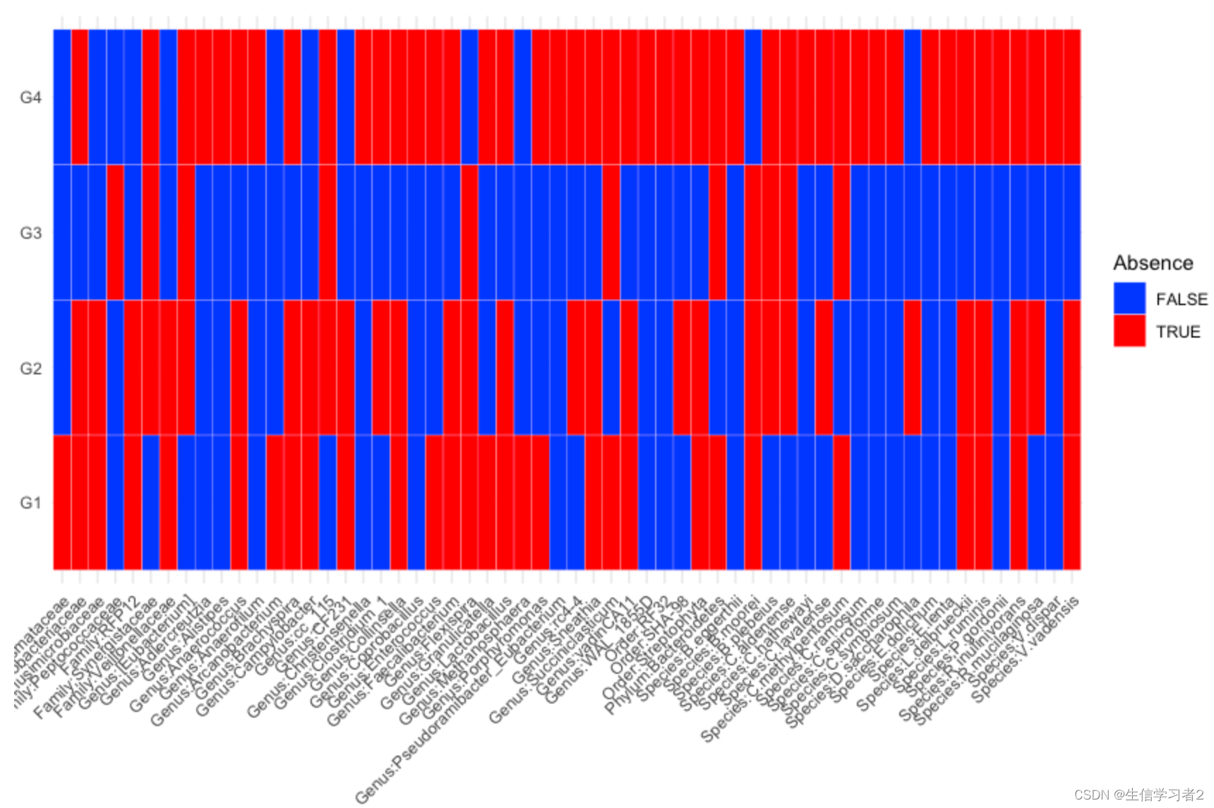
结果:可以看到不同微生物在不同分组的结构零是不一样的。
ANCOM-BC2 trend test
ANCOM-BC2初步结果:
-
lfc: log fold changes obtained from the ANCOM-BC2 log-linear (natural log) model.
-
se: standard errors (SEs) of lfc.
-
W: test statistics. W = lfc/se.
-
p: p-values. P-values are obtained from two-sided Z-test using the test statistic W.
-
q: adjusted p-values. Adjusted p-values are obtained by applying p_adj_method to p.
-
diff: TRUE if the taxon is significant (has q less than alpha).
-
passed_ss: TRUE if the taxon passed the sensitivity analysis, i.e., adding different pseudo-counts to 0s would not change the results.
#| warning: false
#| message: false

res_trend <- primary_ancombc2_species_output$res_trend %>%
  dplyr::rowwise() %>%
  dplyr::filter(grepl("Species:", taxon)|grepl("Genus:", taxon)) %>%
  dplyr::mutate(taxon = ifelse(grepl("Genus:", taxon),
                        paste(strsplit(taxon, ":")[[1]][2], "spp."),
                        strsplit(taxon, ":")[[1]][2])) %>%
  dplyr::ungroup() %>%
  dplyr::filter(p_val < 0.05) %>%
  dplyr::arrange(taxon)

# addWorksheet(wb, "group_species")
# writeData(wb, "group_species", res_trend)

df_fig_group <- res_trend %>%
  dplyr::transmute(taxon,
            fc2 = round(exp(lfc_group1g2), 2),
            fc3 = round(exp(lfc_group1g3), 2),
            fc4 = round(exp(lfc_group1g4), 2),
            p_val, q_val, passed_ss) %>%
  tidyr::pivot_longer(fc2:fc4, names_to = "group", values_to = "value") %>%
  dplyr::mutate(color = ifelse(q_val < 0.05, "seagreen", "black")) %>%
  dplyr::arrange(desc(color))
df_fig_group$group <- recode(df_fig_group$group, `fc2` = "G2",
                            `fc3` = "G3", `fc4` = "G4")

head(df_fig_group[, 1:6])
| taxon | p_val | q_val | passed_ss | group | value |
|---|---|---|---|---|---|
| B.uniformis | 0 | 0 | FALSE | G2 | 0.80 |
| B.uniformis | 0 | 0 | FALSE | G3 | 0.41 |
| B.uniformis | 0 | 0 | FALSE | G4 | 0.35 |
| Bacteroides spp. | 0 | 0 | FALSE | G2 | 0.71 |
| Bacteroides spp. | 0 | 0 | FALSE | G3 | 0.52 |
| Bacteroides spp. | 0 | 0 | FALSE | G4 | 0.25 |
结果:G1组作为Reference group进行多组ANCOMBC-2分析。
HIV-1 infection status at species level
使用ANCOMBC-2算法对HIV-1 infection status分组间微生物species水平进行差异分析。
if (file.exists("./data/GMSB-data/rds/status_ancombc2_species.rds")) {
  status_ancombc2_species_output <- readRDS("./data/GMSB-data/rds/status_ancombc2_species.rds")
} else {

set.seed(123)
status_ancombc2_species_output <- ancombc2(
  data = tse,
  assay_name = "counts",
  tax_level = "Species",
  fix_formula = "status + abx_use",
  rand_formula = NULL,
  p_adj_method = "BY",
  prv_cut = 0.10,
  lib_cut = 1000,
  s0_perc = 0.05,
  group = "status",
  struc_zero = TRUE,
  neg_lb = TRUE,
  alpha = 0.05,
  n_cl = 4,
  verbose = TRUE)

if (!dir.exists("./data/GMSB-data/rds/")) {
  dir.create("./data/GMSB-data/rds/", recursive = TRUE)
}
saveRDS(status_ancombc2_species_output, "./data/GMSB-data/rds/status_ancombc2_species.rds")
}
ANCOM-BC2 trend test
ANCOM-BC2初步结果:
-
lfc: log fold changes obtained from the ANCOM-BC2 log-linear (natural log) model.
-
se: standard errors (SEs) of lfc.
-
W: test statistics. W = lfc/se.
-
p: p-values. P-values are obtained from two-sided Z-test using the test statistic W.
-
q: adjusted p-values. Adjusted p-values are obtained by applying p_adj_method to p.
-
diff: TRUE if the taxon is significant (has q less than alpha).
-
passed_ss: TRUE if the taxon passed the sensitivity analysis, i.e., adding different pseudo-counts to 0s would not change the results.
res_prim <- status_ancombc2_species_output$res %>%
  dplyr::rowwise() %>%
  dplyr::filter(grepl("Species:", taxon)|grepl("Genus:", taxon)) %>%
  dplyr::mutate(taxon = ifelse(grepl("Genus:", taxon),
                        paste(strsplit(taxon, ":")[[1]][2], "spp."),
                        strsplit(taxon, ":")[[1]][2])) %>%
  dplyr::ungroup() %>%
  dplyr::filter(p_statussc < 0.05) %>%
  dplyr::arrange(taxon)

# addWorksheet(wb, "status_species")
# writeData(wb, "status_species", res_prim)

df_fig_status <- res_prim %>%
  dplyr::transmute(taxon,
            group = "Case - Ctrl",
            value = round(exp(lfc_statussc), 2), # exp 函数用于计算自然指数函数的值
            p_statussc, q_statussc, passed_ss_statussc) %>%
  dplyr::mutate(color = ifelse(q_statussc < 0.05, "seagreen", "black")) %>%
  dplyr::arrange(desc(color))

head(df_fig_status[, 1:6])
| taxon | group | value | p_statussc | q_statussc | passed_ss_statussc |
|---|---|---|---|---|---|
| B.caccae | Case - Ctrl | 0.60 | 1.368037e-04 | 0.0087267603 | TRUE |
| B.eggerthii | Case - Ctrl | 0.53 | 3.197272e-06 | 0.0004079102 | FALSE |
| C.spiroforme | Case - Ctrl | 1.78 | 8.546400e-06 | 0.0009086300 | FALSE |
| Dehalobacterium spp. | Case - Ctrl | 1.62 | 3.399664e-05 | 0.0027108225 | FALSE |
| E.cylindroides | Case - Ctrl | 0.57 | 6.152982e-05 | 0.0043611222 | FALSE |
| Methanosphaera spp. | Case - Ctrl | 0.50 | 2.197275e-06 | 0.0003504125 | FALSE |
可视化
对上述两个差异分析的ANCOM-BC2 trend test进行可视化。比较两者共有的微生物在两亚组分析的结果。
# Overlapped taxa
set1 <- base::sort(base::intersect(unique(df_fig_group$taxon), unique(df_fig_status$taxon)))
# Unique taxa
set2 <- base::sort(base::setdiff(unique(df_fig_group$taxon), set1))
set3 <- base::sort(base::setdiff(unique(df_fig_status$taxon), set1))

# ANCOM-BC2 trend test results by group
df_fig_group$taxon <- factor(df_fig_group$taxon, levels = c(set1, set2))
distinct_df <- df_fig_group %>%
  dplyr::select(taxon, color) %>%
  dplyr::distinct()
tax_color <- setNames(distinct_df$color, distinct_df$taxon)[c(set1, set2)]

cell_max <- max(abs(df_fig_group$value))
fig_group_species <- df_fig_group %>%
  ggplot(aes(x = group, y = taxon, fill = value)) +
  geom_tile(color = "black") +
  scale_fill_gradient2(low = "blue", high = "red", mid = "white",
                       na.value = "white", midpoint = 1,
                       limit = c(0, cell_max), name = NULL) +
  geom_text(aes(group, taxon, label = value), color = "black", size = 4) +
  labs(x = NULL, y = NULL, title = NULL) +
  theme_minimal() +
  theme(plot.title = element_text(hjust = 0.5),
        axis.text.y = element_text(color = tax_color))

# ANCOM-BC2 trend test results by status
df_fig_status$taxon <- factor(df_fig_status$taxon, levels = c(set1, set3))
distinct_df <- df_fig_status %>%
  dplyr::select(taxon, color) %>%
  dplyr::distinct()
tax_color <- setNames(distinct_df$color, distinct_df$taxon)[c(set1, set3)]

cell_max <- max(abs(df_fig_status$value))
fig_status_species <- df_fig_status %>%
  ggplot(aes(x = group, y = taxon, fill = value)) +
  geom_tile(color = "black") +
  scale_fill_gradient2(low = "blue", high = "red", mid = "white",
                       na.value = "white", midpoint = 1,
                       limit = c(0, cell_max), name = NULL) +
  geom_text(aes(group, taxon, label = value), color = "black", size = 4) +
  labs(x = NULL, y = NULL, title = NULL) +
  theme_minimal() +
  theme(plot.title = element_text(hjust = 0.5),
        axis.text.y = element_text(color = tax_color))

p_da <- ggarrange(
  fig_group_species, fig_status_species,
  ncol = 2, nrow = 1,
  common.legend = TRUE,
  legend = "right", labels = c("a", "b"))

p_da
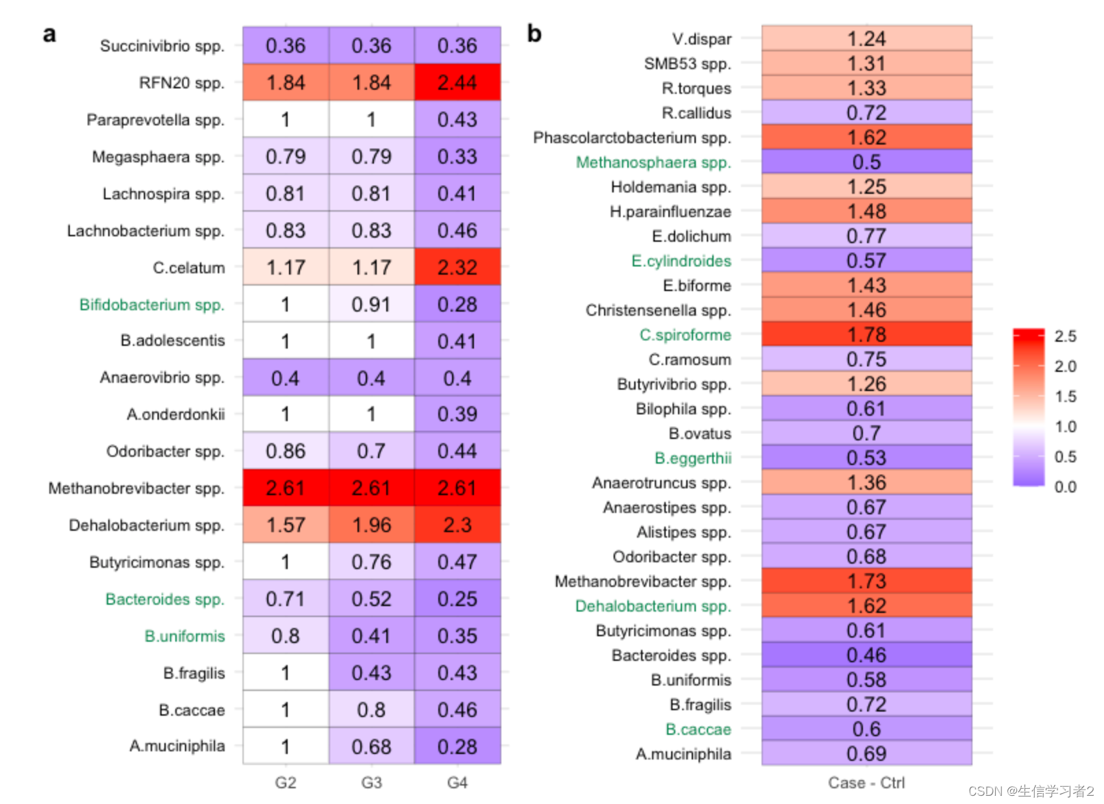
结果:物种在两个分类变量的差异分析结果。
-
数字表示
lfc的自然指数函数的值; -
颜色表示数字从0到2.5渐变,0到1表示
lfc是负数,大于1表示lfc是正数; -
0到1下调,大于1表示上调。
保存数据
# if (!dir.exists("./data/GMSB-data/rds/")) {
#   dir.create("./data/GMSB-data/rds/", recursive = TRUE)
# }
#
# saveRDS(primary_ancombc2_species_output, "./data/GMSB-data/rds/primary_ancombc2_species.rds")
# saveRDS(status_ancombc2_species_output, "./data/GMSB-data/rds/status_ancombc2_species.rds")