文章目录
- 总结
- 参考
- 本门课程的目标
- 机器学习定义
- 从零构建神经网络
- 手写数据集MNIST介绍
- 代码读取数据集MNIST
- 神经网络实现
- 测试手写的图片
- 带有反向查询的神经网络实现
总结
本系列是机器学习课程的系列课程,主要介绍基于python实现神经网络。
参考
BP神经网络及python实现(详细)
本文来源原文链接:https://blog.csdn.net/weixin_66845445/article/details/133828686
用Python从0到1实现一个神经网络(附代码)!
python神经网络编程代码https://gitee.com/iamyoyo/makeyourownneuralnetwork.git
本门课程的目标
完成一个特定行业的算法应用全过程:
懂业务+会选择合适的算法+数据处理+算法训练+算法调优+算法融合
+算法评估+持续调优+工程化接口实现
机器学习定义
关于机器学习的定义,Tom Michael Mitchell的这段话被广泛引用:
对于某类任务T和性能度量P,如果一个计算机程序在T上其性能P随着经验E而自我完善,那么我们称这个计算机程序从经验E中学习。

从零构建神经网络
手写数据集MNIST介绍
mnist_dataset
MNIST数据集是一个包含大量手写数字的集合。 在图像处理领域中,它是一个非常受欢迎的数据集。 经常被用于评估机器学习算法的性能。 MNIST是改进的标准与技术研究所数据库的简称。 MNIST 包含了一个由 70,000 个 28 x 28 的手写数字图像组成的集合,涵盖了从0到9的数字。
本文通过神经网络基于MNIST数据集进行手写识别。
代码读取数据集MNIST
导入库
import numpy
import matplotlib.pyplot
读取mnist_train_100.csv
# open the CSV file and read its contents into a list
data_file = open("mnist_dataset/mnist_train_100.csv", 'r')
data_list = data_file.readlines()
data_file.close()
查看数据集的长度
# check the number of data records (examples)
len(data_list)
# 输出为 100
查看一条数据,这个数据是手写数字的像素值
# show a dataset record
# the first number is the label, the rest are pixel colour values (greyscale 0-255)
data_list[1]
输出为:

需要注意的是,这个字符串的第一个字为真实label,比如
data_list[50]
输出为:
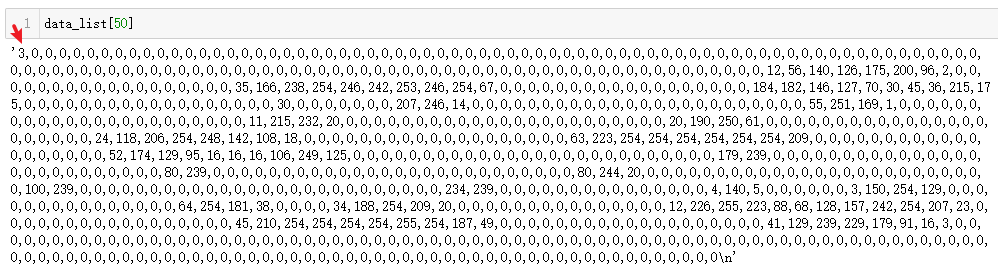
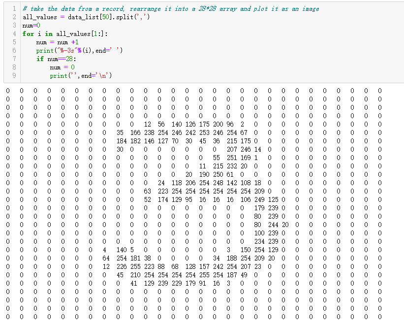
这个输出看不懂,因为这是一个很长的字符串,我们对其进行按照逗号进行分割,然后输出为28*28的,就能看出来了
# take the data from a record, rearrange it into a 28*28 array and plot it as an image
all_values = data_list[50].split(',')
num=0
for i in all_values[1:]:
    num = num +1
    print("%-3s"%(i),end=' ')
    if num==28:
        num = 0
        print('',end='\n')
输出为:
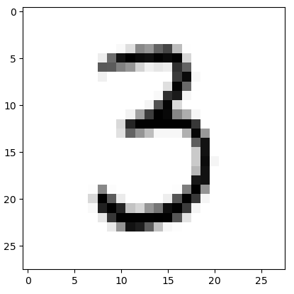
通过用图片的方式查看
# take the data from a record, rearrange it into a 28*28 array and plot it as an image
all_values = data_list[50].split(',')
image_array = numpy.asfarray(all_values[1:]).reshape((28,28))
matplotlib.pyplot.imshow(image_array, cmap='Greys', interpolation='None')
输出为:
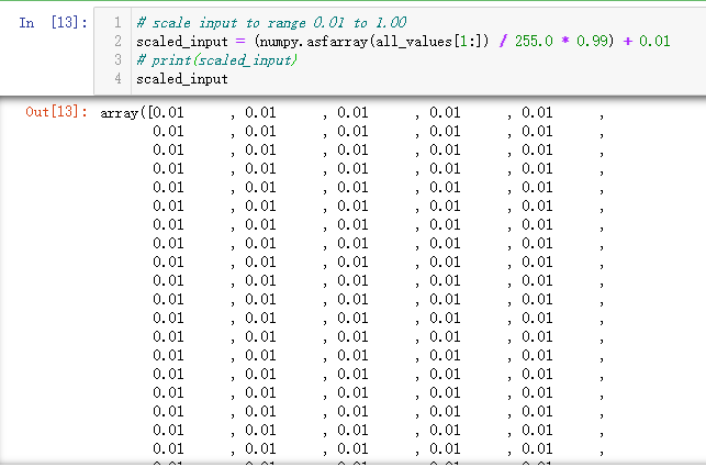
这个像素值为0-255,对其进行归一化操作
# scale input to range 0.01 to 1.00
scaled_input = (numpy.asfarray(all_values[1:]) / 255.0 * 0.99) + 0.01
# print(scaled_input)
scaled_input
输出为:
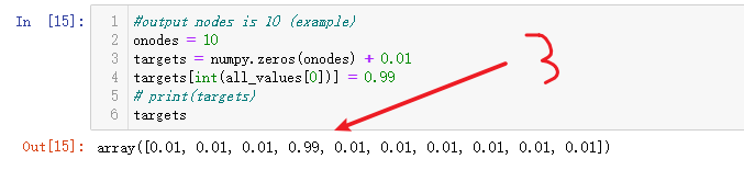
构建一个包含十个输出的标签
#output nodes is 10 (example)
onodes = 10
targets = numpy.zeros(onodes) + 0.01
targets[int(all_values[0])] = 0.99
# print(targets)
targets
输出为:
神经网络实现
导入库
import numpy
# scipy.special for the sigmoid function expit()
import scipy.special
# library for plotting arrays
import matplotlib.pyplot
神经网络实现
# neural network class definition
# 神经网络类定义
class neuralNetwork:
# initialise the neural network
# 初始化神经网络
def __init__(self, inputnodes, hiddennodes, outputnodes, learningrate):
# set number of nodes in each input, hidden, output layer
# 设置每个输入、隐藏、输出层的节点数
self.inodes = inputnodes
self.hnodes = hiddennodes
self.onodes = outputnodes
# link weight matrices, wih and who
# weights inside the arrays are w_i_j, where link is from node i to node j in the next layer
# w11 w21
# w12 w22 etc
# 链接权重矩阵,wih和who
# 数组内的权重w_i_j,链接从节点i到下一层的节点j
# w11 w21
# w12 w22 等等
self.wih = numpy.random.normal(0.0, pow(self.inodes, -0.5), (self.hnodes, self.inodes))
self.who = numpy.random.normal(0.0, pow(self.hnodes, -0.5), (self.onodes, self.hnodes))
# learning rate 学习率
self.lr = learningrate
# activation function is the sigmoid function
# 激活函数是sigmoid函数
self.activation_function = lambda x: scipy.special.expit(x)
pass
# train the neural network
# 训练神经网络
def train(self, inputs_list, targets_list):
# convert inputs list to 2d array
# 将输入列表转换为2d数组
inputs = numpy.array(inputs_list, ndmin=2).T
targets = numpy.array(targets_list, ndmin=2).T
# calculate signals into hidden layer
# 计算输入到隐藏层的信号
hidden_inputs = numpy.dot(self.wih, inputs)
# calculate the signals emerging from hidden layer
# 计算从隐藏层输出的信号
hidden_outputs = self.activation_function(hidden_inputs)
# calculate signals into final output layer
# 计算最终输出层的信号
final_inputs = numpy.dot(self.who, hidden_outputs)
# calculate the signals emerging from final output layer
# 计算从最终输出层输出的信号
final_outputs = self.activation_function(final_inputs)
# output layer error is the (target - actual)
# 输出层误差是(目标 - 实际)
output_errors = targets - final_outputs
# hidden layer error is the output_errors, split by weights, recombined at hidden nodes
# 隐藏层误差是输出层误差,按权重分解,在隐藏节点重新组合
hidden_errors = numpy.dot(self.who.T, output_errors)
# update the weights for the links between the hidden and output layers
# 更新隐藏层和输出层之间的权重
self.who += self.lr * numpy.dot((output_errors * final_outputs * (1.0 - final_outputs)), numpy.transpose(hidden_outputs))
# update the weights for the links between the input and hidden layers
# 更新输入层和隐藏层之间的权重
self.wih += self.lr * numpy.dot((hidden_errors * hidden_outputs * (1.0 - hidden_outputs)), numpy.transpose(inputs))
pass
# query the neural network
# 查询神经网络
def query(self, inputs_list):
# convert inputs list to 2d array
# 将输入列表转换为2d数组
inputs = numpy.array(inputs_list, ndmin=2).T
# calculate signals into hidden layer
# 计算输入到隐藏层的信号
hidden_inputs = numpy.dot(self.wih, inputs)
# calculate the signals emerging from hidden layer
# 计算从隐藏层输出的信号
hidden_outputs = self.activation_function(hidden_inputs)
# calculate signals into final output layer
# 计算最终输出层的信号
final_inputs = numpy.dot(self.who, hidden_outputs)
# calculate the signals emerging from final output layer
# 计算从最终输出层输出的信号
final_outputs = self.activation_function(final_inputs)
return final_outputs
定义参数,并初始化神经网络
# number of input, hidden and output nodes
input_nodes = 784
hidden_nodes = 200
output_nodes = 10

# learning rate
learning_rate = 0.1

# create instance of neural network
n = neuralNetwork(input_nodes,hidden_nodes,output_nodes, learning_rate)
n # <__main__.neuralNetwork at 0x2778590e5e0>
查看数据集
# load the mnist training data CSV file into a list
training_data_file = open("mnist_dataset/mnist_train.csv", 'r')
training_data_list = training_data_file.readlines()
training_data_file.close()
len(training_data_list) # 60001
# 其中第1行为列名 ,后面需要去掉,只保留后60000条
开始训练,该步骤需要等待一会,才能训练完成
# train the neural network
# 训练神经网络
# epochs is the number of times the training data set is used for training
# epochs次数,循环训练5次
epochs = 5

for e in range(epochs):
    # go through all records in the training data set
    # 每次取60000条数据,剔除列名
    for record in training_data_list[1:]:
        # split the record by the ',' commas
        # 用逗号分割
        all_values = record.split(',')
        # scale and shift the inputs
        # 对图像的像素值进行归一化操作
        inputs = (numpy.asfarray(all_values[1:]) / 255.0 * 0.99) + 0.01
        # create the target output values (all 0.01, except the desired label which is 0.99)
        # 创建一个包含十个输出的向量,初始值为0.01
        targets = numpy.zeros(output_nodes) + 0.01
        # all_values[0] is the target label for this record
        # 对 label的 位置设置为0.99
        targets[int(all_values[0])] = 0.99
        # 开始训练
        n.train(inputs, targets)
        pass
    pass
查看训练后的权重
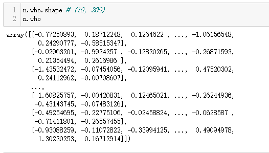
n.who.shape # (10, 200)
n.who
输出为:
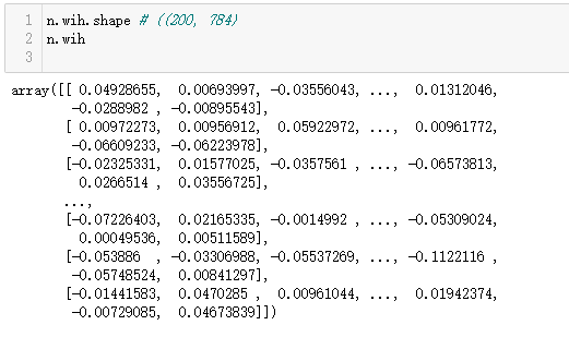
n.wih.shape # ((200, 784)
n.wih
输出为:
查看测试集
# load the mnist test data CSV file into a list
test_data_file = open("mnist_dataset/mnist_test.csv", 'r')
test_data_list = test_data_file.readlines()
test_data_file.close()
len(test_data_list) # 10001
# 其中第1行为列名 ,后面需要去掉,只保留后10000条
预测测试集
# test the neural network
# 测试网络
# scorecard for how well the network performs, initially empty
# 计算网络性能,初始为空
scorecard = []

# go through all the records in the test data set
# 传入所有的测试集
for record in test_data_list[1:]:
    # split the record by the ',' commas
    # 使用逗号分割
    all_values = record.split(',')
    # correct answer is first value
    # 获取当前的测试集的label
    correct_label = int(all_values[0])
    # scale and shift the inputs
    # 归一化操作
    inputs = (numpy.asfarray(all_values[1:]) / 255.0 * 0.99) + 0.01
    # query the network
    # 对测试集进行预测
    outputs = n.query(inputs)
    # the index of the highest value corresponds to the label
    # 获取输出中最大的概率的位置
    label = numpy.argmax(outputs)
    # append correct or incorrect to list
    # 按照预测的正确与否分别填入1和0
    if (label == correct_label):
        # network's answer matches correct answer, add 1 to scorecard
        # 答案匹配正确,输入1
        scorecard.append(1)
    else:
        # network's answer doesn't match correct answer, add 0 to scorecard
        # 答案不匹配,输入0
        scorecard.append(0)
        pass

    pass
计算网络性能
# calculate the performance score, the fraction of correct answers
scorecard_array = numpy.asarray(scorecard)
print ("performance = ", scorecard_array.sum() / scorecard_array.size)
# performance =  0.9725
输出为:
performance = 0.9725
测试手写的图片
导入库
# helper to load data from PNG image files
import imageio.v3
# glob helps select multiple files using patterns
import glob
定义数据集列表
# our own image test data set
our_own_dataset = []
读取多个数据
# glob.glob获取一个可编历对象,使用它可以逐个获取匹配的文件路径名。glob.glob同时获取所有的匹配路径
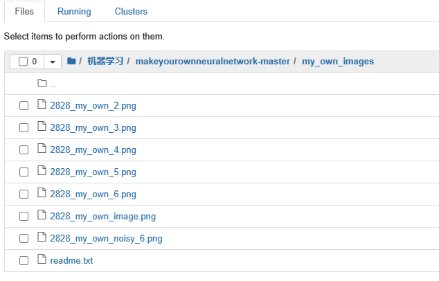
for image_file_name in glob.glob('my_own_images/2828_my_own_?.png'):
# 输出 匹配到的文件
print ("loading ... ", image_file_name)
# use the filename to set the correct label
# 文件名中包含了文件的正确标签
label = int(image_file_name[-5:-4])
# load image data from png files into an array
# 把 图片转换为 文本
img_array = imageio.v3.imread(image_file_name, mode='F')
# reshape from 28x28 to list of 784 values, invert values
# 把28*28的矩阵转换为 784和1维
img_data = 255.0 - img_array.reshape(784)
# then scale data to range from 0.01 to 1.0
# 对数据进行归一化操作,最小值为0.01
img_data = (img_data / 255.0 * 0.99) + 0.01
print(numpy.min(img_data))
print(numpy.max(img_data))
# append label and image data to test data set
# 把 laebl和图片拼接起来
record = numpy.append(label,img_data)
print(record.shape)
# 把封装好的 一维存储在列表中
our_own_dataset.append(record)
pass
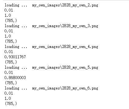
读取的数据如下:
输出为,
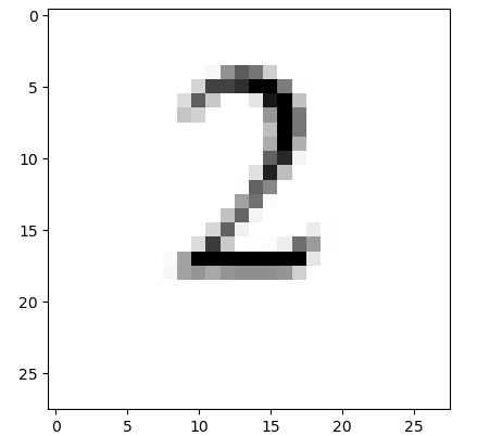
查看手写的图片
matplotlib.pyplot.imshow(our_own_dataset[0][1:].reshape(28,28), cmap='Greys', interpolation='None')
输出为:
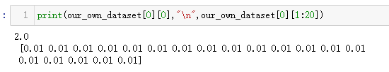
输出对应的像数值
# print(our_own_dataset[0])
print(our_own_dataset[0][0],"\n",our_own_dataset[0][1:20])
输出如下:
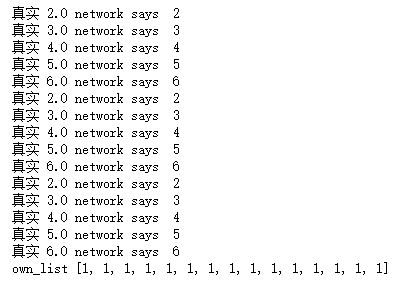
测试手写数据效果
own_list = []
for i in our_own_dataset:
    correct_label = i[0]
    img_data = i[1:]
    # query the network
    outputs = n.query(img_data)
#     print ('outputs预测',outputs)

    # the index of the highest value corresponds to the label
    label = numpy.argmax(outputs)
    print('真实',correct_label,"network says ", label)
    if (label == correct_label):
        # network's answer matches correct answer, add 1 to scorecard
        own_list.append(1)
    else:
        # network's answer doesn't match correct answer, add 0 to scorecard
        own_list.append(0)

print("own_list",own_list)
输出为:
带有反向查询的神经网络实现
该部分代码与 从零构建神经网络大多类似,代码如下:
导入库
import numpy
# scipy.special for the sigmoid function expit(), and its inverse logit()
import scipy.special
# library for plotting arrays
import matplotlib.pyplot
定义带有反向查询的神经网络
# neural network class definition
# 神经网络类定义
class neuralNetwork:


    # initialise the neural network
    # 初始化神经网络
    def __init__(self, inputnodes, hiddennodes, outputnodes, learningrate):
        # set number of nodes in each input, hidden, output layer
        # 设置每个输入、隐藏、输出层的节点数
        self.inodes = inputnodes
        self.hnodes = hiddennodes
        self.onodes = outputnodes

        # link weight matrices, wih and who
        # weights inside the arrays are w_i_j, where link is from node i to node j in the next layer
        # w11 w21
        # w12 w22 etc
        # 链接权重矩阵,wih和who
        # 数组内的权重w_i_j,链接从节点i到下一层的节点j
        # w11 w21
        # w12 w22 等等
        self.wih = numpy.random.normal(0.0, pow(self.inodes, -0.5), (self.hnodes, self.inodes))
        self.who = numpy.random.normal(0.0, pow(self.hnodes, -0.5), (self.onodes, self.hnodes))

        # learning rate 学习率
        self.lr = learningrate

        # activation function is the sigmoid function
        # 激活函数是sigmoid函数
        self.activation_function = lambda x: scipy.special.expit(x)
        self.inverse_activation_function = lambda x: scipy.special.logit(x)

        pass


    # train the neural network
    # 训练神经网络
    def train(self, inputs_list, targets_list):
        # convert inputs list to 2d array
        # 将输入列表转换为2d数组
        inputs = numpy.array(inputs_list, ndmin=2).T
        targets = numpy.array(targets_list, ndmin=2).T

        # calculate signals into hidden layer
        # 计算输入到隐藏层的信号
        hidden_inputs = numpy.dot(self.wih, inputs)
        # calculate the signals emerging from hidden layer
        # 计算从隐藏层输出的信号
        hidden_outputs = self.activation_function(hidden_inputs)

        # calculate signals into final output layer
        # 计算最终输出层的信号
        final_inputs = numpy.dot(self.who, hidden_outputs)
        # calculate the signals emerging from final output layer
        # 计算从最终输出层输出的信号
        final_outputs = self.activation_function(final_inputs)

        # output layer error is the (target - actual)
        # 输出层误差是(目标 - 实际)
        output_errors = targets - final_outputs
        # hidden layer error is the output_errors, split by weights, recombined at hidden nodes
        # 隐藏层误差是输出层误差,按权重分解,在隐藏节点重新组合
        hidden_errors = numpy.dot(self.who.T, output_errors)

        # update the weights for the links between the hidden and output layers
        # 更新隐藏层和输出层之间的权重
        self.who += self.lr * numpy.dot((output_errors * final_outputs * (1.0 - final_outputs)), numpy.transpose(hidden_outputs))

        # update the weights for the links between the input and hidden layers
        # 更新输入层和隐藏层之间的权重
        self.wih += self.lr * numpy.dot((hidden_errors * hidden_outputs * (1.0 - hidden_outputs)), numpy.transpose(inputs))

        pass


    # query the neural network
    # 查询神经网络
    def query(self, inputs_list):
        # convert inputs list to 2d array
        # 将输入列表转换为2d数组
        inputs = numpy.array(inputs_list, ndmin=2).T

        # calculate signals into hidden layer
        # 计算输入到隐藏层的信号
        hidden_inputs = numpy.dot(self.wih, inputs)
        # calculate the signals emerging from hidden layer
        # 计算从隐藏层输出的信号
        hidden_outputs = self.activation_function(hidden_inputs)

        # calculate signals into final output layer
        # 计算最终输出层的信号
        final_inputs = numpy.dot(self.who, hidden_outputs)
        # calculate the signals emerging from final output layer
        # 计算从最终输出层输出的信号
        final_outputs = self.activation_function(final_inputs)

        return final_outputs


    # backquery the neural network
    # we'll use the same termnimology to each item,
    # eg target are the values at the right of the network, albeit used as input
    # eg hidden_output is the signal to the right of the middle nodes
    # 反向 查询
    def backquery(self, targets_list):
        # transpose the targets list to a vertical array
        # 将目标列表转置为垂直数组
        final_outputs = numpy.array(targets_list, ndmin=2).T

        # calculate the signal into the final output layer
        # 计算最终输出层的输入信号
        final_inputs = self.inverse_activation_function(final_outputs)

        # calculate the signal out of the hidden layer
        # 计算隐藏层的输出信号
        hidden_outputs = numpy.dot(self.who.T, final_inputs)
        # scale them back to 0.01 to .99
        # 将隐藏层的输出信号缩放到0.01到0.99之间
        hidden_outputs -= numpy.min(hidden_outputs)
        hidden_outputs /= numpy.max(hidden_outputs)
        hidden_outputs *= 0.98
        hidden_outputs += 0.01

        # calculate the signal into the hidden layer
        # 计算隐藏层的输入信号
        hidden_inputs = self.inverse_activation_function(hidden_outputs)

        # calculate the signal out of the input layer
        # 计算输入层的输出信号
        inputs = numpy.dot(self.wih.T, hidden_inputs)
        # scale them back to 0.01 to .99
        # 将输入层的输出信号缩放到0.01到0.99之间
        inputs -= numpy.min(inputs)
        inputs /= numpy.max(inputs)
        inputs *= 0.98
        inputs += 0.01

        return inputs
初始化神经网络
# number of input, hidden and output nodes
# 定义网络的输入 隐藏 输出节点数量
input_nodes = 784
hidden_nodes = 200
output_nodes = 10

# learning rate
# 学习率
learning_rate = 0.1

# create instance of neural network
# 实例化网络
n = neuralNetwork(input_nodes,hidden_nodes,output_nodes, learning_rate)
加载数据集
# load the mnist training data CSV file into a list
training_data_file = open("mnist_dataset/mnist_train.csv", 'r')
training_data_list = training_data_file.readlines()
training_data_file.close()
训练模型
# train the neural network

# epochs is the number of times the training data set is used for training
epochs = 5

for e in range(epochs):
    print("\n epochs------->",e)
    num = 0
    # go through all records in the training data set
    data_list = len(training_data_list[1:])
    for record in training_data_list[1:]:
        # split the record by the ',' commas
        all_values = record.split(',')
        # scale and shift the inputs
        inputs = (numpy.asfarray(all_values[1:]) / 255.0 * 0.99) + 0.01
        # create the target output values (all 0.01, except the desired label which is 0.99)
        targets = numpy.zeros(output_nodes) + 0.01
        # all_values[0] is the target label for this record
        targets[int(all_values[0])] = 0.99
        n.train(inputs, targets)
        num +=1
        if num %500==0:
            print("\r epochs {} 当前进度为 {}".format(e,num/data_list),end="")
        pass
    pass
输出为:
epochs-------> 0
epochs 0 当前进度为 1.091666666666666744
epochs-------> 1
epochs 1 当前进度为 1.091666666666666744
epochs-------> 2
epochs 2 当前进度为 1.091666666666666744
epochs-------> 3
epochs 3 当前进度为 1.091666666666666744
epochs-------> 4
epochs 4 当前进度为 1.091666666666666744
加载测试数据
# load the mnist test data CSV file into a list
test_data_file = open("mnist_dataset/mnist_test.csv", 'r')
test_data_list = test_data_file.readlines()
test_data_file.close()
加载测试数据
# test the neural network

# scorecard for how well the network performs, initially empty
scorecard = []

# go through all the records in the test data set
for record in test_data_list[1:]:
    # split the record by the ',' commas
    all_values = record.split(',')
    # correct answer is first value
    correct_label = int(all_values[0])
    # scale and shift the inputs
    inputs = (numpy.asfarray(all_values[1:]) / 255.0 * 0.99) + 0.01
    # query the network
    outputs = n.query(inputs)
    # the index of the highest value corresponds to the label
    label = numpy.argmax(outputs)
    # append correct or incorrect to list
    if (label == correct_label):
        # network's answer matches correct answer, add 1 to scorecard
        scorecard.append(1)
    else:
        # network's answer doesn't match correct answer, add 0 to scorecard
        scorecard.append(0)
        pass

    pass
计算模型性能
# calculate the performance score, the fraction of correct answers
scorecard_array = numpy.asarray(scorecard)
print ("performance = ", scorecard_array.sum() / scorecard_array.size)
# performance =  0.9737
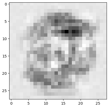
根据模型反向生成图片
# run the network backwards, given a label, see what image it produces

# label to test
label = 0
# create the output signals for this label
targets = numpy.zeros(output_nodes) + 0.01
# all_values[0] is the target label for this record
targets[label] = 0.99
print(targets)

# get image data
image_data = n.backquery(targets)

# plot image data
matplotlib.pyplot.imshow(image_data.reshape(28,28), cmap='Greys', interpolation='None')
输出为: