使用MATLAB快速对波形进行傅里叶分解到有限次谐波
目录
- 使用MATLAB快速对波形进行傅里叶分解到有限次谐波
- 1、解析表达式分解到有限次谐波
- 1.1、理论分析
- 1.2、全部代码
- 2、数值波形分解到有限次谐波
- 2.1、基础理论
- 2.2、对应代码
很多时候对功率放大器设计阻抗空间的分析都是从波形开始的,那么如何 从波形得到其对应的谐波分量呢? 如何从单纯的波形得到设计所需的阻抗呢?答案就是傅里叶分解啦。
波形的分解一般分为两个情况,其一就是纯粹的解析表达式,如连续F类的波形:
V
C
−
F
=
(
1
−
2
3
cos
θ
)
2
⋅
(
1
+
1
3
cos
θ
)
⋅
(
1
−
γ
sin
θ
)
I
C
−
F
=
1
π
+
1
2
cos
θ
+
2
3
π
cos
(
2
θ
)
\begin{aligned} &{V_{C-F}} = {\left( {1 - \frac{2}{{\sqrt 3 }}\cos \theta } \right)^2} \cdot \left( {1 + \frac{1}{{\sqrt 3 }}\cos \theta } \right) \cdot (1 - \gamma \sin \theta )\\ &{I_{C-F}} = \frac{1}{\pi } + \frac{1}{2}\cos \theta + \frac{2}{{3\pi }}\cos (2\theta ) \end{aligned}
VC−F=(1−32cosθ)2⋅(1+31cosθ)⋅(1−γsinθ)IC−F=π1+21cosθ+3π2cos(2θ)
这种情况是相对非常直观的,对式子进行展开化简约分就能得到最终的结果,但是三角函数相乘化简也是非常的麻烦。
另一种情况就是数值表达式的波形,其解析表达式可能非常复杂难求,只能使用具有有限数值点进行求解,如考虑到无限次谐波的EF类的波形(图中是每1°一个数据,电压电流都是具有360大小的向量数据):

对于这种情况,需要使用离散的傅里叶级数进行求解了,需要大量的计算,可以使用matlab来进行简化。
1、解析表达式分解到有限次谐波
1.1、理论分析
可以使用傅里叶级数进行分解:
f
(
t
)
=
a
0
2
+
a
1
c
o
s
(
ω
t
)
+
b
1
s
i
n
(
ω
t
)
+
a
2
c
o
s
(
2
ω
t
)
+
b
2
s
i
n
(
2
ω
t
)
+
.
.
.
=
a
0
2
+
∑
n
=
1
∞
[
a
n
c
o
s
(
n
ω
t
)
+
b
n
s
i
n
(
n
ω
t
)
]
\begin{aligned} f(t)& =\frac{a_0}2+a_1cos(\omega t)+b_1sin(\omega t) \\ &+a_2cos(2\omega t)+b_2sin(2\omega t) \\ &+... \\ &=\frac{a_0}2+\sum_{n=1}^\infty\left[a_ncos(n\omega t)+b_nsin(n\omega t)\right] \end{aligned}
f(t)=2a0+a1cos(ωt)+b1sin(ωt)+a2cos(2ωt)+b2sin(2ωt)+...=2a0+n=1∑∞[ancos(nωt)+bnsin(nωt)]
使用积分计算其中的傅里叶参数:
a
n
=
2
T
∫
t
0
t
0
+
T
f
(
t
)
c
o
s
(
n
ω
t
)
d
t
b
n
=
2
T
∫
t
0
t
0
+
T
f
(
t
)
s
i
n
(
n
ω
t
)
d
t
\begin{aligned}a_n&=\frac{2}{T}\int_{t_0}^{t_0+T}f(t)cos(n\omega t)dt\\b_n&=\frac{2}{T}\int_{t_0}^{t_0+T}f(t)sin(n\omega t)dt\end{aligned}
anbn=T2∫t0t0+Tf(t)cos(nωt)dt=T2∫t0t0+Tf(t)sin(nωt)dt
积分计算其中的傅里叶参数对应代码,周期T=2*pi:
disp('开始求取电流傅里叶分解数值');
I_A0=int(i_theta/pi,theta,int_i_low,int_i_high);
Fouier=I_A0/2;
for n=1:order
    I_A(n)=(int(i_theta*cos(n*theta)/pi,theta,int_i_low,int_i_high));
    I_B(n)=(int(i_theta*sin(n*theta)/pi,theta,int_i_low,int_i_high));
    Fouier=Fouier+I_A(n)*cos(n*theta)+I_B(n)*sin(n*theta);
end
disp(Fouier)


disp('开始求取电压傅里叶分解数值');
V_A0=int(v_theta/pi,theta,int_v_low,int_v_high);
Fouier=V_A0/2;
for n=1:order
    V_A(n)=(int(v_theta*cos(n*theta)/pi,theta,int_v_low,int_v_high));
    V_B(n)=(int(v_theta*sin(n*theta)/pi,theta,int_v_low,int_v_high));
    Fouier=Fouier+V_A(n)*cos(n*theta)+V_B(n)*sin(n*theta);
end
disp(Fouier)
使用电流电压的傅里叶参数可以计算最终波形对应的阻抗:
Z
n
,
f
=
−
a
V
,
n
+
j
b
V
,
n
a
I
,
n
+
j
b
I
,
n
{Z_{n,f}} =- \frac{{{a_{V,n}} + j{b_{V,n}}}}{{{a_{I,n}} + j{b_{I,n}}}}
Zn,f=−aI,n+jbI,naV,n+jbV,n
阻抗计算对应代码(阻抗参考是Ropt,因此要乘以0.5,具体参考Ropt定义):
% 阻抗参考是Ropt,因此要乘以0.5
disp('最佳阻抗');
for n=1:order
    disp(simplify(-0.5*(V_A(n)+1j*V_B(n))/(I_A(n)+1j*I_B(n))));
end
可以看到,对于上面的连续F类,得到的结果为:
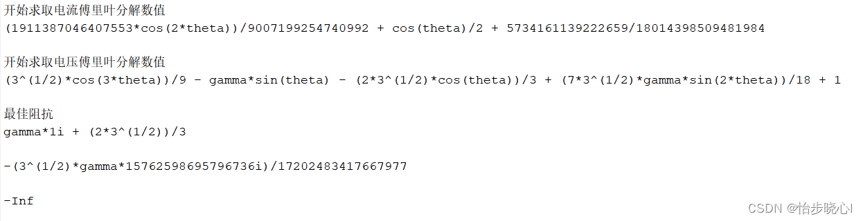
和理论结果一致:
{
Z
l
f
,
C
−
F
=
(
2
3
+
j
γ
)
R
o
p
t
Z
2
f
,
C
−
F
=
−
j
7
3
π
24
R
o
p
t
Z
3
f
,
C
−
F
=
∞
\begin{cases}Z_{\mathrm{l}f,C-F}=\left(\frac{2}{\sqrt{3}}+j\gamma\right)R_{opt}\\Z_{2f,C-F}=-j\frac{7\sqrt{3}\pi}{24}R_{opt}\\\\Z_{3f,C-F}=\infty\end{cases}
⎩
⎨
⎧Zlf,C−F=(32+jγ)RoptZ2f,C−F=−j2473πRoptZ3f,C−F=∞
1.2、全部代码
clear all
close all
clc
syms theta gamma


v_theta=(1-2/(sqrt(3))*cos(theta))^2*(1+1/(sqrt(3))*cos(theta))*(1-gamma*sin(theta));
i_theta=1/pi+1/2*cos(theta)+2/(3*pi)*cos(2*theta);

order=3;
int_i_low=0;
int_i_high=2*pi;
int_v_low=0;
int_v_high=2*pi;


disp('开始求取电流傅里叶分解数值');
I_A0=int(i_theta/pi,theta,int_i_low,int_i_high);
Fouier=I_A0/2;
for n=1:order
    I_A(n)=(int(i_theta*cos(n*theta)/pi,theta,int_i_low,int_i_high));
    I_B(n)=(int(i_theta*sin(n*theta)/pi,theta,int_i_low,int_i_high));
    Fouier=Fouier+I_A(n)*cos(n*theta)+I_B(n)*sin(n*theta);
end
disp(Fouier)


disp('开始求取电压傅里叶分解数值');
V_A0=int(v_theta/pi,theta,int_v_low,int_v_high);
Fouier=V_A0/2;
for n=1:order
    V_A(n)=(int(v_theta*cos(n*theta)/pi,theta,int_v_low,int_v_high));
    V_B(n)=(int(v_theta*sin(n*theta)/pi,theta,int_v_low,int_v_high));
    Fouier=Fouier+V_A(n)*cos(n*theta)+V_B(n)*sin(n*theta);
end
disp(Fouier)

% 阻抗参考Ropt,因此要乘以0.5
disp('最佳阻抗');
for n=1:order
    disp(simplify(-0.5*(V_A(n)+1j*V_B(n))/(I_A(n)+1j*I_B(n))));
end
2、数值波形分解到有限次谐波
2.1、基础理论
我们现在只知道离散个点的波形点,如上面的EF类的波形,也就是0-360度对应的电压电流纵坐标:
v_theta=[0	0	0	0	0	0	0	0	0	0	0	0	0	0	0	0	0	0	0	0	0	0	0	0	0	0	0	0	0	0	0	0	0	0	0	0	0	0	0	0	0	0	0	0	0	0	0	0	0	0	0	0	0	0	0	0	0	0	0	0	0	0	0	0	0	0	0	0	0	0	0	0	0	0	0	0	0	0	0	0	0	0	0	0	0	0	0	0	0	0	0	0	0	0	0	0	0	0	0	0	0	0	0	0	0	0	0	0	0	0	0	0	0	0	0	0	0	0	0	0	0	0	0	0	0	0	0	0	0	0	0	0	0	0	0	0	0	0	0	0	0	0	0	0	0	0.129750090188117	0.255289136488565	0.376625563240092	0.493771567461190	0.606743078675062	0.715559714306197	0.820244730715221	0.920824969944700	1.01733080225395	1.10979606452633	1.19825799463809	1.28275716188279	1.36333739355047	1.44004569776601	1.51293218269540	1.58204997223385	1.64745511829383	1.70920650981569	1.76736577862760	1.82199720228559	1.87316760402839	1.92094624998539	1.96540474377936	2.00661691866925	2.04465872738108	2.07960812977794	2.11154497852306	2.14055090289194	2.16670919089223	2.19010466985182	2.21082358563754	2.22895348066865	2.24458307089029	2.25780212187380	2.26870132421120	2.27737216837235	2.28390681919350	2.28839799016632	2.29093881769660	2.29162273550150	2.29054334931401	2.28779431206257	2.28346919969278	2.27766138779744	2.27046392921947	2.26196943279093	2.25226994336973	2.24145682333331	2.22962063568691	2.21685102894105	2.20323662391102	2.18886490258756	2.17382209922559	2.15819309379440	2.14206130792919	2.12550860352063	2.10861518407504	2.09145949897413	2.07411815075892	2.05666580555838	2.03917510677888	2.02171659216579	2.00435861434412	1.98716726494012	1.97020630238054	1.95353708346157	1.93721849877388	1.92130691206479	1.90585610361357	1.89091721768970	1.87653871415869	1.86276632429423	1.84964301084941	1.83720893243417	1.82550141223995	1.81455491114661	1.80440100524056	1.79506836776717	1.78658275553402	1.77896699977591	1.77224100148585	1.76642173121067	1.76152323330329	1.75755663461776	1.75453015762705	1.75244913793754	1.75131604616785	1.75113051415408	1.75188936543721	1.75358664998267	1.75621368307635	1.75975908833542	1.76420884476677	1.76954633780040	1.77575241421946	1.78280544090333	1.79068136729513	1.79935379149957	1.80879402991220	1.81897119027659	1.82985224806066	1.84140212603937	1.85358377696624	1.86635826921214	1.87968487524548	1.89352116282429	1.90782308876684	1.92254509516368	1.93764020789113	1.95306013728256	1.96875538081114	1.98467532763490	2.00076836485232	2.01698198531430	2.03326289683643	2.04955713265309	2.06581016295376	2.08196700733989	2.09797234803965	2.11377064371706	2.12930624371044	2.14452350253532	2.15936689448609	2.17378112817058	2.18771126081174	2.20110281215137	2.21390187779056	2.22605524180278	2.23751048845669	2.24821611288614	2.25812163054717	2.26717768530275	2.27533615597819	2.28255026123205	2.28877466258980	2.29396556548978	2.29808081819375	2.30108000841734	2.30292455753854	2.30357781224585	2.30300513349109	2.30117398261556	2.29805400452179	2.29361710776788	2.28783754146454	2.28069196886001	2.27215953750263	2.26222194587468	2.25086350639677	2.23807120470647	2.22383475512025	2.20814665219245	2.19100221829117	2.17239964711551	2.15234004308466	2.13082745653473	2.10786891466503	2.08347444818129	2.05765711358891	2.03043301109573	2.00182129808950	1.97184419816107	1.94052700565101	1.90789808570285	1.87398886981256	1.83883384687003	1.80247054969468	1.76493953707278	1.72628437131108	1.68655159132716	1.64579068130262	1.60405403493198	1.56139691530578	1.51787741047259	1.47355638473006	1.42849742570208	1.38276678726365	1.33643332838164	1.28956844794501	1.24224601566347	1.19454229911915	1.14653588706108	1.09830760903752	1.04994045146629	1.00151947024801	0.953131700032240	0.904866060251106	0.856813258039101	0.809065688162828	0.761717330088043	0.714863642315586	0.668601454121624	0.623028854841491	0.578245080839374	0.534350400309946	0.491445996060881	0.449633846428079	0.409016604478074	0.369697475654887	0.331780094030513	0.295368397320433	0.260566500827536	0.227478570479249	0.196208695124241	0.166860758256219	0.139538309333334	0.114344434862345	0.0913816294174346	0.0707516667636549	0.0525554712551816	0.0368929896782647	0.0238630637086112	0.0135633031520352	0.00608996013661750	0.00153780442336330];
i_theta=[2.71877140023093e-15	0.0105802447184730	0.0214593627914783	0.0326318770606530	0.0440919543587784	0.0558334102470919	0.0678497141808513	0.0801339950975745	0.0926790474218736	0.105477337480283	0.118521010318992	0.131801896916889	0.145311521785851	0.159041110949733	0.172981600293053	0.187123644269917	0.201457624963267	0.215973661484159	0.230661619700282	0.245511122282607	0.260511559058602	0.275652097660105	0.290921694453584	0.306309105740139	0.321802899212305	0.337391465654379	0.353063030872676	0.368805667841881	0.384607309053348	0.400455759050972	0.416338707140022	0.432243740254109	0.448158355965254	0.464069975621858	0.479965957599197	0.495833610646935	0.511660207318022	0.527432997463224	0.543139221775473	0.558766125368123	0.574300971371190	0.589731054529576	0.605043714787323	0.620226350841903	0.635266433652606	0.650151519887139	0.664869265290589	0.679407437961026	0.693753931516094	0.707896778135093	0.721824161461166	0.735524429348392	0.748986106438761	0.762197906554188	0.775148744888967	0.787827749988275	0.800224275498601	0.812327911676234	0.824128496640252	0.835616127356703	0.846781170341063	0.857614272066312	0.868106369064369	0.878248697708976	0.888032803668483	0.897450551017397	0.906494130995960	0.915156070407433	0.923429239643184	0.931306860326153	0.938782512563674	0.945850141801153	0.952504065268514	0.958738978011872	0.964549958503340	0.969932473822392	0.974882384402731	0.979395948339108	0.983469825249066	0.987101079685117	0.990287184093406	0.993026021315432	0.995315886629956	0.997155489332780	0.998543953852620	0.999480820401845	0.999966045161431	1	0.999583471727408	0.998717660883866	0.997404180066151	0.995645051793016	0.993442705912439	0.990799976553921	0.987720098629568	0.984206703888232	0.980263816527522	0.975895848369025	0.971107593602574	0.965904223105957	0.960291278346913	0.954274664874798	0.947860645409769	0.941055832537829	0.933867181020519	0.926301979728526	0.918367843208913	0.910072702896094	0.901424797977131	0.892432665922306	0.883105132692350	0.873451302634046	0.863480548076357	0.853202498639505	0.842627030269838	0.831764254013592	0.820624504542979	0.809218328448336	0.797556472310320	0.785649870566400	0.773509633186142	0.761147033169997	0.748573493886507	0.735800576263023	0.722839965845228	0.709703459740842	0.696402953463102	0.682950427689634	0.669357934952504	0.655637586275242	0.641801537772738	0.627861977229913	0.613831110675097	0.599721148964041	0.585544294390456	0.571312727338955	0.557038592996174	0.542733988135819	0.528410947993227	0.514081433244961	0.499757317108799	0.485450372579319	0.471172259814115	0.456934513685486	0	0	0	0	0	0	0	0	0	0	0	0	0	0	0	0	0	0	0	0	0	0	0	0	0	0	0	0	0	0	0	0	0	0	0	0	0	0	0	0	0	0	0	0	0	0	0	0	0	0	0	0	0	0	0	0	0	0	0	0	0	0	0	0	0	0	0	0	0	0	0	0	0	0	0	0	0	0	0	0	0	0	0	0	0	0	0	0	0	0	0	0	0	0	0	0	0	0	0	0	0	0	0	0	0	0	0	0	0	0	0	0	0	0	0	0	0	0	0	0	0	0	0	0	0	0	0	0	0	0	0	0	0	0	0	0	0	0	0	0	0	0	0	0	0	0	0	0	0	0	0	0	0	0	0	0	0	0	0	0	0	0	0	0	0	0	0	0	0	0	0	0	0	0	0	0	0	0	0	0	0	0	0	0	0	0	0	0	0	0	0	0	0	0	0	0	0	0	0	0	0	0	0	0	0	0	0	0	0	0	0	0	0	0	0	0;]
此时需要使用离散傅里叶级数进行傅里叶分量的计算,理论公式如:
可以使用傅里叶级数进行分解:
f
(
t
)
=
a
0
2
+
a
1
c
o
s
(
ω
t
)
+
b
1
s
i
n
(
ω
t
)
+
a
2
c
o
s
(
2
ω
t
)
+
b
2
s
i
n
(
2
ω
t
)
+
.
.
.
=
a
0
2
+
∑
n
=
1
∞
[
a
n
c
o
s
(
n
ω
t
)
+
b
n
s
i
n
(
n
ω
t
)
]
\begin{aligned} f(t)& =\frac{a_0}2+a_1cos(\omega t)+b_1sin(\omega t) \\ &+a_2cos(2\omega t)+b_2sin(2\omega t) \\ &+... \\ &=\frac{a_0}2+\sum_{n=1}^\infty\left[a_ncos(n\omega t)+b_nsin(n\omega t)\right] \end{aligned}
f(t)=2a0+a1cos(ωt)+b1sin(ωt)+a2cos(2ωt)+b2sin(2ωt)+...=2a0+n=1∑∞[ancos(nωt)+bnsin(nωt)]
使用求和计算其中的傅里叶参数:
a
n
=
2
N
∑
f
(
θ
)
c
o
s
(
n
θ
)
d
θ
b
n
=
2
N
∑
f
(
θ
)
sin
(
n
θ
)
d
θ
\begin{array}{l} {a_n} = \frac{2}{N}\sum {f(\theta )cos(n\theta )d\theta } \\ {b_n} = \frac{2}{N}\sum {f(\theta )\sin (n\theta )d\theta } \end{array}
an=N2∑f(θ)cos(nθ)dθbn=N2∑f(θ)sin(nθ)dθ
对应代码:
disp('开始求取电流傅里叶分解数值');
I_A0=sum(i_theta)/(length(theta_num))*2;
Fouier=I_A0/2;
for n=1:order
    I_A(n)=2*sum(i_theta.*cos(n*theta_num))/(length(theta_num));
    I_B(n)=2*sum(i_theta.*sin(n*theta_num))/(length(theta_num));
    Fouier=Fouier+I_A(n)*cos(n*theta)+I_B(n)*sin(n*theta);
end
disp(vpa(Fouier))
使用上面的EF类带入,得到结果为(2次谐波短路,三次谐波开路,画Smith圆图匹配时由于匹配方向问题需要对阻抗取共轭):
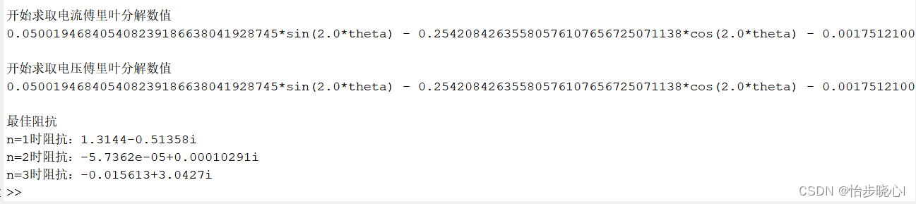
结果和理论一致。
2.2、对应代码
clear all
close all
clc
syms theta


theta_num=(0:pi/180:2*pi-pi/180);
% 连续F类,相乘变量,自由因子
% gamma=0;
% v_theta=((1-2/(sqrt(3)).*cos(theta_num)).^2).*(1+1/(sqrt(3)).*cos(theta_num)).*(1-gamma.*sin(theta_num));
% i_theta=1/pi+1/2*cos(theta_num)+2/(3*pi)*cos(2*theta_num);
% EF类波形
v_theta=[0	0	0	0	0	0	0	0	0	0	0	0	0	0	0	0	0	0	0	0	0	0	0	0	0	0	0	0	0	0	0	0	0	0	0	0	0	0	0	0	0	0	0	0	0	0	0	0	0	0	0	0	0	0	0	0	0	0	0	0	0	0	0	0	0	0	0	0	0	0	0	0	0	0	0	0	0	0	0	0	0	0	0	0	0	0	0	0	0	0	0	0	0	0	0	0	0	0	0	0	0	0	0	0	0	0	0	0	0	0	0	0	0	0	0	0	0	0	0	0	0	0	0	0	0	0	0	0	0	0	0	0	0	0	0	0	0	0	0	0	0	0	0	0	0	0.129750090188117	0.255289136488565	0.376625563240092	0.493771567461190	0.606743078675062	0.715559714306197	0.820244730715221	0.920824969944700	1.01733080225395	1.10979606452633	1.19825799463809	1.28275716188279	1.36333739355047	1.44004569776601	1.51293218269540	1.58204997223385	1.64745511829383	1.70920650981569	1.76736577862760	1.82199720228559	1.87316760402839	1.92094624998539	1.96540474377936	2.00661691866925	2.04465872738108	2.07960812977794	2.11154497852306	2.14055090289194	2.16670919089223	2.19010466985182	2.21082358563754	2.22895348066865	2.24458307089029	2.25780212187380	2.26870132421120	2.27737216837235	2.28390681919350	2.28839799016632	2.29093881769660	2.29162273550150	2.29054334931401	2.28779431206257	2.28346919969278	2.27766138779744	2.27046392921947	2.26196943279093	2.25226994336973	2.24145682333331	2.22962063568691	2.21685102894105	2.20323662391102	2.18886490258756	2.17382209922559	2.15819309379440	2.14206130792919	2.12550860352063	2.10861518407504	2.09145949897413	2.07411815075892	2.05666580555838	2.03917510677888	2.02171659216579	2.00435861434412	1.98716726494012	1.97020630238054	1.95353708346157	1.93721849877388	1.92130691206479	1.90585610361357	1.89091721768970	1.87653871415869	1.86276632429423	1.84964301084941	1.83720893243417	1.82550141223995	1.81455491114661	1.80440100524056	1.79506836776717	1.78658275553402	1.77896699977591	1.77224100148585	1.76642173121067	1.76152323330329	1.75755663461776	1.75453015762705	1.75244913793754	1.75131604616785	1.75113051415408	1.75188936543721	1.75358664998267	1.75621368307635	1.75975908833542	1.76420884476677	1.76954633780040	1.77575241421946	1.78280544090333	1.79068136729513	1.79935379149957	1.80879402991220	1.81897119027659	1.82985224806066	1.84140212603937	1.85358377696624	1.86635826921214	1.87968487524548	1.89352116282429	1.90782308876684	1.92254509516368	1.93764020789113	1.95306013728256	1.96875538081114	1.98467532763490	2.00076836485232	2.01698198531430	2.03326289683643	2.04955713265309	2.06581016295376	2.08196700733989	2.09797234803965	2.11377064371706	2.12930624371044	2.14452350253532	2.15936689448609	2.17378112817058	2.18771126081174	2.20110281215137	2.21390187779056	2.22605524180278	2.23751048845669	2.24821611288614	2.25812163054717	2.26717768530275	2.27533615597819	2.28255026123205	2.28877466258980	2.29396556548978	2.29808081819375	2.30108000841734	2.30292455753854	2.30357781224585	2.30300513349109	2.30117398261556	2.29805400452179	2.29361710776788	2.28783754146454	2.28069196886001	2.27215953750263	2.26222194587468	2.25086350639677	2.23807120470647	2.22383475512025	2.20814665219245	2.19100221829117	2.17239964711551	2.15234004308466	2.13082745653473	2.10786891466503	2.08347444818129	2.05765711358891	2.03043301109573	2.00182129808950	1.97184419816107	1.94052700565101	1.90789808570285	1.87398886981256	1.83883384687003	1.80247054969468	1.76493953707278	1.72628437131108	1.68655159132716	1.64579068130262	1.60405403493198	1.56139691530578	1.51787741047259	1.47355638473006	1.42849742570208	1.38276678726365	1.33643332838164	1.28956844794501	1.24224601566347	1.19454229911915	1.14653588706108	1.09830760903752	1.04994045146629	1.00151947024801	0.953131700032240	0.904866060251106	0.856813258039101	0.809065688162828	0.761717330088043	0.714863642315586	0.668601454121624	0.623028854841491	0.578245080839374	0.534350400309946	0.491445996060881	0.449633846428079	0.409016604478074	0.369697475654887	0.331780094030513	0.295368397320433	0.260566500827536	0.227478570479249	0.196208695124241	0.166860758256219	0.139538309333334	0.114344434862345	0.0913816294174346	0.0707516667636549	0.0525554712551816	0.0368929896782647	0.0238630637086112	0.0135633031520352	0.00608996013661750	0.00153780442336330];
i_theta=[2.71877140023093e-15	0.0105802447184730	0.0214593627914783	0.0326318770606530	0.0440919543587784	0.0558334102470919	0.0678497141808513	0.0801339950975745	0.0926790474218736	0.105477337480283	0.118521010318992	0.131801896916889	0.145311521785851	0.159041110949733	0.172981600293053	0.187123644269917	0.201457624963267	0.215973661484159	0.230661619700282	0.245511122282607	0.260511559058602	0.275652097660105	0.290921694453584	0.306309105740139	0.321802899212305	0.337391465654379	0.353063030872676	0.368805667841881	0.384607309053348	0.400455759050972	0.416338707140022	0.432243740254109	0.448158355965254	0.464069975621858	0.479965957599197	0.495833610646935	0.511660207318022	0.527432997463224	0.543139221775473	0.558766125368123	0.574300971371190	0.589731054529576	0.605043714787323	0.620226350841903	0.635266433652606	0.650151519887139	0.664869265290589	0.679407437961026	0.693753931516094	0.707896778135093	0.721824161461166	0.735524429348392	0.748986106438761	0.762197906554188	0.775148744888967	0.787827749988275	0.800224275498601	0.812327911676234	0.824128496640252	0.835616127356703	0.846781170341063	0.857614272066312	0.868106369064369	0.878248697708976	0.888032803668483	0.897450551017397	0.906494130995960	0.915156070407433	0.923429239643184	0.931306860326153	0.938782512563674	0.945850141801153	0.952504065268514	0.958738978011872	0.964549958503340	0.969932473822392	0.974882384402731	0.979395948339108	0.983469825249066	0.987101079685117	0.990287184093406	0.993026021315432	0.995315886629956	0.997155489332780	0.998543953852620	0.999480820401845	0.999966045161431	1	0.999583471727408	0.998717660883866	0.997404180066151	0.995645051793016	0.993442705912439	0.990799976553921	0.987720098629568	0.984206703888232	0.980263816527522	0.975895848369025	0.971107593602574	0.965904223105957	0.960291278346913	0.954274664874798	0.947860645409769	0.941055832537829	0.933867181020519	0.926301979728526	0.918367843208913	0.910072702896094	0.901424797977131	0.892432665922306	0.883105132692350	0.873451302634046	0.863480548076357	0.853202498639505	0.842627030269838	0.831764254013592	0.820624504542979	0.809218328448336	0.797556472310320	0.785649870566400	0.773509633186142	0.761147033169997	0.748573493886507	0.735800576263023	0.722839965845228	0.709703459740842	0.696402953463102	0.682950427689634	0.669357934952504	0.655637586275242	0.641801537772738	0.627861977229913	0.613831110675097	0.599721148964041	0.585544294390456	0.571312727338955	0.557038592996174	0.542733988135819	0.528410947993227	0.514081433244961	0.499757317108799	0.485450372579319	0.471172259814115	0.456934513685486	0	0	0	0	0	0	0	0	0	0	0	0	0	0	0	0	0	0	0	0	0	0	0	0	0	0	0	0	0	0	0	0	0	0	0	0	0	0	0	0	0	0	0	0	0	0	0	0	0	0	0	0	0	0	0	0	0	0	0	0	0	0	0	0	0	0	0	0	0	0	0	0	0	0	0	0	0	0	0	0	0	0	0	0	0	0	0	0	0	0	0	0	0	0	0	0	0	0	0	0	0	0	0	0	0	0	0	0	0	0	0	0	0	0	0	0	0	0	0	0	0	0	0	0	0	0	0	0	0	0	0	0	0	0	0	0	0	0	0	0	0	0	0	0	0	0	0	0	0	0	0	0	0	0	0	0	0	0	0	0	0	0	0	0	0	0	0	0	0	0	0	0	0	0	0	0	0	0	0	0	0	0	0	0	0	0	0	0	0	0	0	0	0	0	0	0	0	0	0	0	0	0	0	0	0	0	0	0	0	0	0	0	0	0	0	0;]

% 分析到的阶数
order=3;


disp('开始求取电流傅里叶分解数值');
I_A0=sum(i_theta)/(length(theta_num))*2;
Fouier=I_A0/2;
for n=1:order
    I_A(n)=2*sum(i_theta.*cos(n*theta_num))/(length(theta_num));
    I_B(n)=2*sum(i_theta.*sin(n*theta_num))/(length(theta_num));
    Fouier=Fouier+I_A(n)*cos(n*theta)+I_B(n)*sin(n*theta);
end
disp(vpa(Fouier))


disp('开始求取电压傅里叶分解数值');
I_V0=sum(v_theta)/(length(theta_num))*2;
Fouier=I_V0/2;
for n=1:order
    V_A(n)=2*sum(v_theta.*cos(n*theta_num))/(length(theta_num));
    V_B(n)=2*sum(v_theta.*sin(n*theta_num))/(length(theta_num));
    Fouier=Fouier+I_A(n)*cos(n*theta)+I_B(n)*sin(n*theta);
end
disp(vpa(Fouier))


disp('最佳阻抗');
for n=1:order
    tmp=(-0.5*(V_A(n)+1j*V_B(n))./(I_A(n)+1j*I_B(n)));
    disp(['n=',num2str(n),'时阻抗:',num2str(tmp)]);
end
% 注意!!!画Smith圆图匹配时由于匹配方向问题需要对阻抗取共轭