#2.2挑选term---

selected_clusterenrich=enrichmets[grepl(pattern = "cilium|matrix|excular|BMP|inflamm|development|muscle|
                                        vaso|pulmonary|alveoli",
                                        x = enrichmets$Description),]

head(selected_clusterenrich) 

distinct(selected_clusterenrich)

# remove duplicate rows based on Description 并且保留其他所有变量
distinct_df <- distinct(enrichmets, Description,.keep_all = TRUE)

library(ggplot2)
ggplot( distinct_df %>%
         dplyr::filter(stringr::str_detect(pattern = "cilium|matrix|excular|BMP|inflamm|development|muscle",Description))  %>%
         group_by(Description) %>%
         add_count()  %>%
         dplyr::arrange(dplyr::desc(n),dplyr::desc(Description)) %>%
         mutate(Description =forcats:: fct_inorder(Description))
       
       , #fibri|matrix|colla
       aes(Cluster, Description)) +
  geom_point(aes(fill=p.adjust, size=Count), shape=21)+
  theme_bw()+
  theme(axis.text.x=element_text(angle=90,hjust = 1,vjust=0.5),
        axis.text.y=element_text(size = 12),
        axis.text = element_text(color = 'black', size = 12)
  )+
  scale_fill_gradient(low="red",high="blue")+
  labs(x=NULL,y=NULL)
# coord_flip()

head(enrichmets)

ggplot( distinct(enrichmets,Description,.keep_all=TRUE)  %>% 
        #  dplyr::mutate(Cluster = factor(Cluster, levels = unique(.$Cluster))) %>%
           
          dplyr::mutate(Description = factor(Description, levels = unique(.$Description))) %>%
        #  dplyr::group_by(Cluster)  %>%
         dplyr::filter(stringr::str_detect(pattern = "cilium organization|motile cilium|cilium movemen|cilium assembly|
                                           cell-matrix adhesion|extracellular matrix organization|regulation of acute inflammatory response to antigenic stimulus|
                                           collagen-containing extracellular matrix|negative regulation of BMP signaling pathway|
                                           extracellular matrix structural constituent|extracellular matrix binding|fibroblast proliferation|
                                           collagen biosynthetic process|collagen trimer|fibrillar collagen trimer|inflammatory response to antigenic stimulus|
                                           chemokine activity|chemokine production|cell chemotaxis|chemoattractant activity|
                                           NLRP3 inflammasome complex assembly|inflammatory response to wounding|Wnt signaling pathway|response to oxidative stress|
                                           regulation of vascular associated smooth muscle cell proliferation|
                                           venous blood vessel development|regulation of developmental growth|lung alveolus development|myofibril assembly|
                                           blood vessel diameter maintenance|
                                           gas transport|cell maturation|regionalization|oxygen carrier activity|oxygen binding|
                                           vascular associated smooth muscle cell proliferation",Description))     %>%
       #  group_by(Description) %>%
         add_count()  %>%
         dplyr::arrange(dplyr::desc(n),dplyr::desc(Description))  %>%
        mutate(Description =forcats:: fct_inorder(Description))
       
       , #fibri|matrix|colla
       aes(Cluster, y = Description)) +  #stringr:: str_wrap
  geom_point(aes(fill=p.adjust, size=Count), shape=21)+
  theme_bw()+
  theme(axis.text.x=element_text(angle=90,hjust = 1,vjust=0.5),
        axis.text.y=element_text(size = 12),
        axis.text = element_text(color = 'black', size = 12)
  )+
  scale_fill_gradient(low="red",high="blue")+
  labs(x=NULL,y=NULL)
# coord_flip()
print(getwd())



p=ggplot( distinct(enrichmets,Description,.keep_all=TRUE)  %>%
            
            dplyr::mutate(Description = factor(Description, levels = unique(.$Description))) %>%  #调整terms显示顺序
            dplyr::filter(stringr::str_detect(pattern = "cilium organization|motile cilium|cilium movemen|cilium assembly|
                                           cell-matrix adhesion|extracellular matrix organization|regulation of acute inflammatory response to antigenic stimulus|
                                           collagen-containing extracellular matrix|negative regulation of BMP signaling pathway|
                                           extracellular matrix structural constituent|extracellular matrix binding|fibroblast proliferation|
                                           collagen biosynthetic process|collagen trimer|fibrillar collagen trimer|inflammatory response to antigenic stimulus|
                                           chemokine activity|chemokine production|cell chemotaxis|chemoattractant activity|
                                           NLRP3 inflammasome complex assembly|inflammatory response to wounding|Wnt signaling pathway|response to oxidative stress|
                                           regulation of vascular associated smooth muscle cell proliferation|
                                           venous blood vessel development|regulation of developmental growth|lung alveolus development|myofibril assembly|
                                           blood vessel diameter maintenance|
                                           gas transport|cell maturation|regionalization|oxygen carrier activity|oxygen binding|
                                           vascular associated smooth muscle cell proliferation",Description))  %>%
            group_by(Description) %>%
            add_count()  %>%
            dplyr::arrange(dplyr::desc(n),dplyr::desc(Description)) %>%
            mutate(Description =forcats:: fct_inorder(Description))
          
          , #fibri|matrix|colla
          aes(Cluster, y = Description)) +  #stringr:: str_wrap
  #scale_y_discrete(labels = function(x) stringr::str_wrap(x, width = 60)) +  #调整terms长度
  geom_point(aes(fill=p.adjust, size=Count), shape=21)+
  theme_bw()+
  theme(axis.text.x=element_text(angle=90,hjust = 1,vjust=0.5),
        axis.text.y=element_text(size = 12),
        axis.text = element_text(color = 'black', size = 12)
  )+
  scale_fill_gradient(low="red",high="blue")+
  labs(x=NULL,y=NULL)
# coord_flip()
print(getwd())




ggsave(filename ="~/silicosis/spatial/sp_cluster_rigions_after_harmony/enrichents12.pdf",plot = p,
       width = 10,height = 12,limitsize = FALSE)



######展示term内所有基因，用热图展示-------

#提取画图的数据
  
p$data


#提取图形中的所有基因-----
mygenes=  p$data $geneID %>% stringr::str_split(.,"/",simplify = TRUE)  %>%as.vector()   %>%unique()
frame_for_genes=p$data %>%as.data.frame() %>% dplyr::group_by(Cluster)  #后面使用split的话，必须按照分组排序
head(frame_for_genes)

my_genelist=  split(frame_for_genes, frame_for_genes$Cluster, drop = TRUE)  %>%  #注意drop参数的理解

  lapply(function(x) select(x, geneID));my_genelist
                  


my_genelist=  split(frame_for_genes, frame_for_genes$Cluster, drop = TRUE)  %>%  #注意drop参数的理解
  
  lapply(function(x) x$geneID);my_genelist

mygenes=my_genelist %>% lapply( function(x)  {stringr::str_split(x,"/",simplify = TRUE)  %>%as.vector()   %>%unique()}   )

#准备画热图，加载seurat对象
load("/home/data/t040413/silicosis/spatial_transcriptomics/silicosis_ST_harmony_SCT_r0.5.rds")
{dim(d.all)
  DefaultAssay(d.all)="Spatial"
  #visium_slides=SplitObject(object = d.all,split.by = "stim")
  
  names(d.all);dim(d.all)
  d.all@meta.data %>%head()
  head(colnames(d.all))
  #1 给d.all 添加meta信息------
  adata_obs=read.csv("~/silicosis/spatial/adata_obs.csv")
  head(adata_obs)
  mymeta=  paste0(d.all@meta.data$orig.ident,"_",colnames(d.all))  %>% gsub("-.*","",.)  # %>%  head()
  head(mymeta)
  tail(mymeta)
  
  #掉-及其之后内容
  adata_obs$col= adata_obs$spot_id %>% gsub("-.*","",.)    # %>%  head()
  head(adata_obs)
  
  rownames(adata_obs)=adata_obs$col
  adata_obs=adata_obs[mymeta,]
  head(adata_obs)
  identical(mymeta,adata_obs$col)
  d.all=AddMetaData(d.all,metadata = adata_obs)
  head(d.all@meta.data)}

##构建画热图对象---
Idents(d.all)=d.all$clusters
a=AverageExpression(d.all,return.seurat = TRUE)
a$orig.ident=rownames(a@meta.data)
head(a@meta.data)
head(markers)

rownames(a) %>%head()
head(mygenes)
table(mygenes %in% rownames(a))
DoHeatmap(a,draw.lines = FALSE, slot = 'scale.data', group.by = 'orig.ident',
          features = mygenes ) + 
  ggplot2:: scale_color_discrete(name = "Identity", labels =  unique(a$orig.ident) %>%sort()  )



##doheatmap做出来的图不好调整，换成heatmap自己调整

p=DoHeatmap(a,draw.lines = FALSE, slot = 'scale.data', group.by = 'orig.ident',
          features = mygenes ) + 
  ggplot2:: scale_color_discrete( labels =  unique(a$orig.ident) %>%sort()  ) #name = "Identity",

p$data %>%head()


##########这种方式容易出现bug，不建议------
if (F) {
  
    wide_data <- p$data %>% .[,-4] %>%
      tidyr:: pivot_wider(names_from = Cell, values_from = Expression)
    
    print(wide_data)  
    
    mydata=  wide_data %>%
      dplyr:: select(-Feature) %>%
      as.matrix()
    head(mydata)
    rownames(mydata)=wide_data$Feature
    mydata=mydata[,c("Bronchial zone", "Fibrogenic zone",   "Interstitial zone",  "Inflammatory zone","Vascular zone"  )]
    
    p2=pheatmap::  pheatmap(mydata, fontsize_row = 2, 
                            clustering_method = "ward.D2",
                            #     annotation_col = wide_data$Feature,
                            annotation_colors = c("Interstitial zone" = "red", "Bronchial zone" = "blue", "Fibrogenic zone" = "green", "Vascular zone" = "purple") ,
                            cluster_cols = FALSE,
                            column_order = c("Inflammatory zone", "Vascular zone"  ,"Bronchial zone", "Fibrogenic zone"   )
    )
    
    getwd()
    ggplot2::ggsave(filename = "~/silicosis/spatial/sp_cluster_rigions_after_harmony/heatmap_usingpheatmap.pdf",width = 8,height = 10,limitsize = FALSE,plot = p2)
    
    
   
}



##########建议如下方式画热图------
a$orig.ident=a@meta.data %>%rownames()
a@meta.data %>%head()
Idents(a)=a$orig.ident
 
a@assays$Spatial@scale.data  %>%head()

mydata=a@assays$Spatial@scale.data
mydata=mydata[rownames(mydata) %in% (mygenes %>%unlist() %>%unique()) ,]
mydata= mydata[,c( "Fibrogenic zone",  "Inflammatory zone",   "Bronchial zone","Interstitial zone","Vascular zone"  )]
head(mydata)
p3=pheatmap::  pheatmap(mydata, fontsize_row = 2,  
                    clustering_method = "ward.D2",
                    #     annotation_col = wide_data$Feature,
                    annotation_colors = c("Interstitial zone" = "red", "Bronchial zone" = "blue", "Fibrogenic zone" = "green", "Vascular zone" = "purple") ,
                    cluster_cols = FALSE,
                    column_order = c("Inflammatory zone", "Vascular zone"  ,"Bronchial zone", "Fibrogenic zone"   )
)

getwd()
ggplot2::ggsave(filename = "~/silicosis/spatial/sp_cluster_rigions_after_harmony/heatmap_usingpheatmap2.pdf",width = 8,height = 10,limitsize = FALSE,plot = p3)



#########单独画出炎症区和纤维化区---------
a@assays$Spatial@scale.data  %>%head()

mydata=a@assays$Spatial@scale.data
mygenes2= my_genelist[c('Inflammatory zone','Fibrogenic zone')] %>%  unlist() %>% stringr::str_split("/",simplify = TRUE) 

mydata2=mydata[rownames(mydata) %in% ( mygenes2 %>%unlist() %>%unique()) ,]
mydata2= mydata2[,c( "Fibrogenic zone",  "Inflammatory zone" )]
head(mydata2)

p3=pheatmap::  pheatmap(mydata2, fontsize_row = 5,  #scale = 'row',
                         clustering_method = "ward.D2",
                        #     annotation_col = wide_data$Feature,
                        annotation_colors = c("Interstitial zone" = "red", "Bronchial zone" = "blue", "Fibrogenic zone" = "green", "Vascular zone" = "purple") ,
                        cluster_cols = FALSE,
                        column_order = c("Inflammatory zone", "Vascular zone"  ,"Bronchial zone", "Fibrogenic zone"   )
)

getwd()
ggplot2::ggsave(filename = "~/silicosis/spatial/sp_cluster_rigions_after_harmony/heatmap_usingpheatmap3.pdf",width = 4,height = 8,limitsize = FALSE,plot = p3)

.libPaths(c("/home/data/t040413/R/x86_64-pc-linux-gnu-library/4.2",
            "/home/data/t040413/R/yll/usr/local/lib/R/site-library", 
            "/usr/local/lib/R/library",
            "/refdir/Rlib/"))

library(Seurat)
library(ggplot2)
library(dplyr)
load('/home/data/t040413/silicosis/fibroblast_myofibroblast2/subset_data_fibroblast_myofibroblast2.rds')



print(getwd())
dir.create("~/silicosis/fibroblast_myofibroblast2/slilica_fibroblast_enrichments")
setwd("~/silicosis/fibroblast_myofibroblast2/slilica_fibroblast_enrichments")
getwd()

DimPlot(subset_data,label = TRUE)

markers_foreach=FindAllMarkers(subset_data,only.pos = TRUE,densify = TRUE)
head(markers_foreach)



all_degs=markers_foreach
markers=markers_foreach

#install.packages("AnnotationDbi")
#BiocManager::install(version = '3.18')
#BiocManager::install('AnnotationDbi',version = '3.18')
{
  ##########################---------------------批量富集分析findallmarkers-enrichment analysis==================================================
  #https://mp.weixin.qq.com/s/WyT-7yKB9YKkZjjyraZdPg
  
  
  df=all_degs
  ##筛选阈值确定：p＜0.05，|log2FC|＞1
  p_val_adj = 0.05
  # avg_log2FC = 0.1
  
  fc=seq(0.8,1.4,0.2)
  print(getwd())
  #setwd("../")
  
  for (avg_log2FC in fc) {
    
  #  avg_log2FC=0.5
    
    dir.create(paste0(avg_log2FC,"/"))
    setwd(paste0(avg_log2FC,"/"))
    
    
    print(getwd())
    print(paste0("Start----",avg_log2FC))
    
    head(all_degs)
    #根据阈值添加上下调分组标签：
    df$direction <- case_when(
      df$avg_log2FC > avg_log2FC & df$p_val_adj < p_val_adj ~ "up",
      df$avg_log2FC < -avg_log2FC & df$p_val_adj < p_val_adj ~ "down",
      TRUE ~ 'none'
    )
    head(df)
    
    df=df[df$direction!="none",]
    head(df)
    dim(df)
    df$mygroup=paste(df$group,df$direction,sep = "_")
    head(df)
    dim(df)
    ##########################----------------------enrichment analysis=
    #https://mp.weixin.qq.com/s/WyT-7yKB9YKkZjjyraZdPg
    {
      library(clusterProfiler)
      library(org.Hs.eg.db) #人
      library(org.Mm.eg.db) #鼠
      library(ggplot2)
      # degs_for_nlung_vs_tlung$gene=rownames(degs_for_nlung_vs_tlung)
      head(markers)
      df=markers %>%dplyr::group_by(cluster)%>%
        filter(p_val_adj <0.05
        )
      sce.markers=df
      head(sce.markers)
      print(getwd())
      ids <- suppressWarnings(bitr(sce.markers$gene, 'SYMBOL', 'ENTREZID', 'org.Mm.eg.db'))
      head(ids)
      
      head(sce.markers)
      tail(sce.markers)
      dim(sce.markers)
      sce.markers=merge(sce.markers,ids,by.x='gene',by.y='SYMBOL')
      head(sce.markers)
      dim(sce.markers)
      sce.markers$group=sce.markers$cluster
      sce.markers=sce.markers[sce.markers$group!="none",]
      dim(sce.markers)
      head(sce.markers)
      getwd()
      #    sce.markers=openxlsx::read.xlsx("/home/data/t040413/silicosis/fibroblast_myofibroblast/group_enrichments/")
      #sce.markers$cluster=sce.markers$mygroup
      dim(sce.markers)
      head(sce.markers)
      gcSample=split(sce.markers$ENTREZID, sce.markers$cluster)
      
      library(clusterProfiler)
      gcSample # entrez id , compareCluster 
      print("===========开始go= All ont===========")
      xx <- compareCluster(gcSample, fun="enrichGO",OrgDb="org.Mm.eg.db" ,   #'org.Hs.eg.db',
                           pvalueCutoff=0.05) #organism="hsa",
      
      
      xx.BP <- compareCluster(gcSample, fun="enrichGO",OrgDb="org.Mm.eg.db" ,   #'org.Hs.eg.db',
                              pvalueCutoff=0.05,readable=TRUE,
                              ont="BP") #organism="hsa",
      p=clusterProfiler::dotplot(object = xx.BP,showCategory = 20,
                                 label_format =60) 
      p=p+ theme(axis.text.x = element_text(angle = 90, 
                                            vjust = 0.5, hjust=0.5))
      p
      ggsave(paste0(avg_log2FC,'_degs_compareCluster-BP_enrichment--3.pdf'),plot = p,width = 13,height = 40,limitsize = F)
      ggsave(paste0(avg_log2FC,'_degs_compareCluster-BP_enrichment--3.pdf'),plot = p,width = 13,height = 40,limitsize = F)
      
      xx.CC <- compareCluster(gcSample, fun="enrichGO",OrgDb="org.Mm.eg.db" ,   #'org.Hs.eg.db',
                              pvalueCutoff=0.05,readable=TRUE,
                              ont="CC") #organism="hsa",
      p=clusterProfiler::dotplot(object = xx.CC,showCategory = 20,
                                 label_format =60) 
      p=p+ theme(axis.text.x = element_text(angle = 90, 
                                            vjust = 0.5, hjust=0.5))
      p
      ggsave(paste0(avg_log2FC,'_degs_compareCluster-CC_enrichment--3.pdf'),plot = p,width = 13,height = 40,limitsize = F)
      ggsave(paste0(avg_log2FC,'_degs_compareCluster-CC_enrichment--3.pdf'),plot = p,width = 13,height = 40,limitsize = F)
      
      xx.MF <- compareCluster(gcSample, fun="enrichGO",OrgDb="org.Mm.eg.db" ,   #'org.Hs.eg.db',
                              pvalueCutoff=0.05,readable=TRUE,
                              ont="MF") #organism="hsa",
      p=clusterProfiler::dotplot(object = xx.MF,showCategory = 20,
                                 label_format =60) 
      p=p+ theme(axis.text.x = element_text(angle = 90, 
                                            vjust = 0.5, hjust=0.5))
      p
      ggsave(paste0(avg_log2FC,'_degs_compareCluster-MF_enrichment--3.pdf'),plot = p,width = 13,height = 40,limitsize = F)
      ggsave(paste0(avg_log2FC,'_degs_compareCluster-MF_enrichment--3.pdf'),plot = p,width = 13,height = 40,limitsize = F)
      
      
      
      print(getwd())
      
      .libPaths()
      
      
      print("===========开始 kegg All ont============")
      gg<-clusterProfiler::compareCluster(gcSample,fun = "enrichKEGG",  #readable=TRUE,
                                          keyType = 'kegg',  #KEGG 富集
                                          organism='mmu',#"rno",
                                          pvalueCutoff = 0.05 #指定 p 值阈值（可指定 1 以输出全部
      )
      
      p=clusterProfiler::dotplot(object = xx,showCategory = 20,
                                 label_format =100) 
      p=p+ theme(axis.text.x = element_text(angle = 90, 
                                            vjust = 0.5, hjust=0.5))
      p
      ggsave(paste0(avg_log2FC,'_degs_compareCluster-GO_enrichment--3.pdf'),plot = p,width = 13,height = 40,limitsize = F)
      ggsave(paste0(avg_log2FC,'_degs_compareCluster-GO_enrichment--3.pdf'),plot = p,width = 13,height = 40,limitsize = F)
      
      xx
      write.csv(xx,file = paste0(avg_log2FC,"compareCluster-GO_enrichment.csv"))
      
      p=clusterProfiler::dotplot(gg,showCategory = 20,
                                 label_format = 40) 
      p4=p+ theme(axis.text.x = element_text(angle = 90, 
                                             vjust = 0.5, hjust=0.5))
      p4
      print(paste("保存位置",getwd(),sep = "  :   "))
      ggsave(paste0(avg_log2FC,'_degs_compareCluster-KEGG_enrichment-2.pdf'),plot = p4,width = 13,height = 25,limitsize = F)
      ggsave(paste0(avg_log2FC,'_degs_compareCluster-KEGG_enrichment-2.pdf'),plot = p4,width = 13,height = 25,limitsize = F)
      
      gg
      openxlsx::write.xlsx(gg,file = paste0(avg_log2FC,"_compareCluster-KEGG_enrichment.xlsx"))
      
      getwd()
      openxlsx::write.xlsx(sce.markers,file = paste0(avg_log2FC,"_sce.markers_for_each_clusterfor_enrichment.xlsx"))
      
      
      ##放大图片
      {
        getwd()
        #bp
        p=clusterProfiler::dotplot(object = xx.BP,showCategory = 100,
                                   label_format =60) 
        p=p+ theme(axis.text.x = element_text(angle = 90, 
                                              vjust = 0.5, hjust=0.5))
        p
        ggsave(paste0(avg_log2FC,'_degs_compareCluster-BP_enrichment-100terms-3.pdf'),plot = p,width = 13,height = 100,limitsize = F)
        ggsave(paste0(avg_log2FC,'_degs_compareCluster-BP_enrichment-100terms-3.pdf'),plot = p,width = 13,height = 100,limitsize = F)
        print((getwd()))
        
        #cc
        p=clusterProfiler::dotplot(object = xx.CC,showCategory = 100,
                                   label_format =60) 
        p=p+ theme(axis.text.x = element_text(angle = 90, 
                                              vjust = 0.5, hjust=0.5))
        p
        ggsave(paste0(avg_log2FC,'_degs_compareCluster-CC_enrichment-100terms-3.pdf'),plot = p,width = 13,height = 100,limitsize = F)
        ggsave(paste0(avg_log2FC,'_degs_compareCluster-CC_enrichment-100terms-3.pdf'),plot = p,width = 13,height = 100,limitsize = F)
        print((getwd()))
        
        #MF
        p=clusterProfiler::dotplot(object = xx.MF,showCategory = 100,
                                   label_format =60) 
        p=p+ theme(axis.text.x = element_text(angle = 90, 
                                              vjust = 0.5, hjust=0.5))
        p
        ggsave(paste0(avg_log2FC,'_degs_compareCluster-MF_enrichment-100terms-3.pdf'),plot = p,width = 13,height = 100,limitsize = F)
        ggsave(paste0(avg_log2FC,'_degs_compareCluster-MF_enrichment-100terms-3.pdf'),plot = p,width = 13,height = 100,limitsize = F)
        print((getwd()))
        
        
        #KEGG
        p=clusterProfiler::dotplot(object = gg,showCategory = 100,
                                   label_format =60) 
        p=p+ theme(axis.text.x = element_text(angle = 90, 
                                              vjust = 0.5, hjust=0.5))
        p
        ggsave(paste0(avg_log2FC,'_degs_compareCluster-KEGG_enrichment-100terms-3.pdf'),plot = p,width = 13,height = 100,limitsize = F)
        ggsave(paste0(avg_log2FC,'_degs_compareCluster-KEGG_enrichment-100terms-3.pdf'),plot = p,width = 13,height = 100,limitsize = F)
        print((getwd()))
        
        
        
      }
      
      #   save(xx.BP,xx.CC,xx.MF, gg, file = "~/silicosis/spatial_transcriptomicsharmony_cluster_0.5res_gsea/xx.Rdata")
      
      xx.BP@compareClusterResult$oncology="BP"
      xx.CC@compareClusterResult$oncology="CC"
      xx.MF@compareClusterResult$oncology="MF"
      
      
      xx.all=do.call(rbind,list(xx.BP@compareClusterResult,
                                xx.CC@compareClusterResult,
                                xx.MF@compareClusterResult))
      head(xx.all)    
      openxlsx::write.xlsx(xx.all,file = paste0(avg_log2FC,"_enrichments_all.xlsx"))    
      
      # save(xx.BP,xx.CC,xx.MF,xx.all,sce.markers,merged_degs, gg, file = "./xx.Rdata")
      
      result <- tryCatch({
        save(xx.BP,xx.CC,xx.MF,xx.all,sce.markers,merged_degs, gg, file = paste0(avg_log2FC,"_xx.Rdata"))
        # 在这里添加你希望在没有报错时执行的代码
        print("没有报错")
      }, error = function(e) {
        print(getwd())  # 在报错时执行的代码
        
        # 在这里添加你希望在报错时执行的额外代码
        save(xx.BP,xx.CC,xx.MF,xx.all,sce.markers, gg, file = paste0(avg_log2FC,"_xx_all.Rdata"))
      })
      
      # print(result)
      
      
      
      
      print(getwd())
      if (F) { 
        #大鼠
        print("===========开始go============")
        xx <-clusterProfiler::compareCluster(gcSample, fun="enrichGO",OrgDb="org.Rn.eg.db",
                                             readable=TRUE,
                                             ont = 'ALL',  #GO Ontology，可选 BP、MF、CC，也可以指定 ALL 同时计算 3 者
                                             pvalueCutoff=0.05) #organism="hsa", #'org.Hs.eg.db',
        
        print("===========开始 kegg============")
        gg<-clusterProfiler::compareCluster(gcSample,fun = "enrichKEGG",
                                            keyType = 'kegg',  #KEGG 富集
                                            organism="rno",
                                            pvalueCutoff = 0.05 #指定 p 值阈值（可指定 1 以输出全部
        )
        
        p=dotplot(xx) 
        p2=p+ theme(axis.text.x = element_text(angle = 90, 
                                               vjust = 0.5, hjust=0.5))
        p2
        ggsave('degs_compareCluster-GO_enrichment-2.pdf',plot = p2,width = 6,height = 20,limitsize = F)
        xx
        openxlsx::write.xlsx(xx,file = "compareCluster-GO_enrichment.xlsx")
        #
        p=dotplot(gg) 
        p4=p+ theme(axis.text.x = element_text(angle = 90, 
                                               vjust = 0.5, hjust=0.5))
        p4
        print(paste("保存位置",getwd(),sep = "  :   "))
        ggsave('degs_compareCluster-KEGG_enrichment-2.pdf',plot = p4,width = 6,height = 12,limitsize = F)
        gg
        openxlsx::write.xlsx(gg,file = "compareCluster-KEGG_enrichment.xlsx")   
      }  
      
      setwd("../")
    }
    
  }
  
  
  
  
}

print(getwd())
#setwd('../')


load("~/silicosis/fibroblast_myofibroblast2/slilica_fibroblast_enrichments/1/1_xx_all.Rdata")




# remove duplicate rows based on Description 并且保留其他所有变量
xx.all<- distinct(xx.all, Description,.keep_all = TRUE)

enrichmets=xx.all

#2.2挑选term---

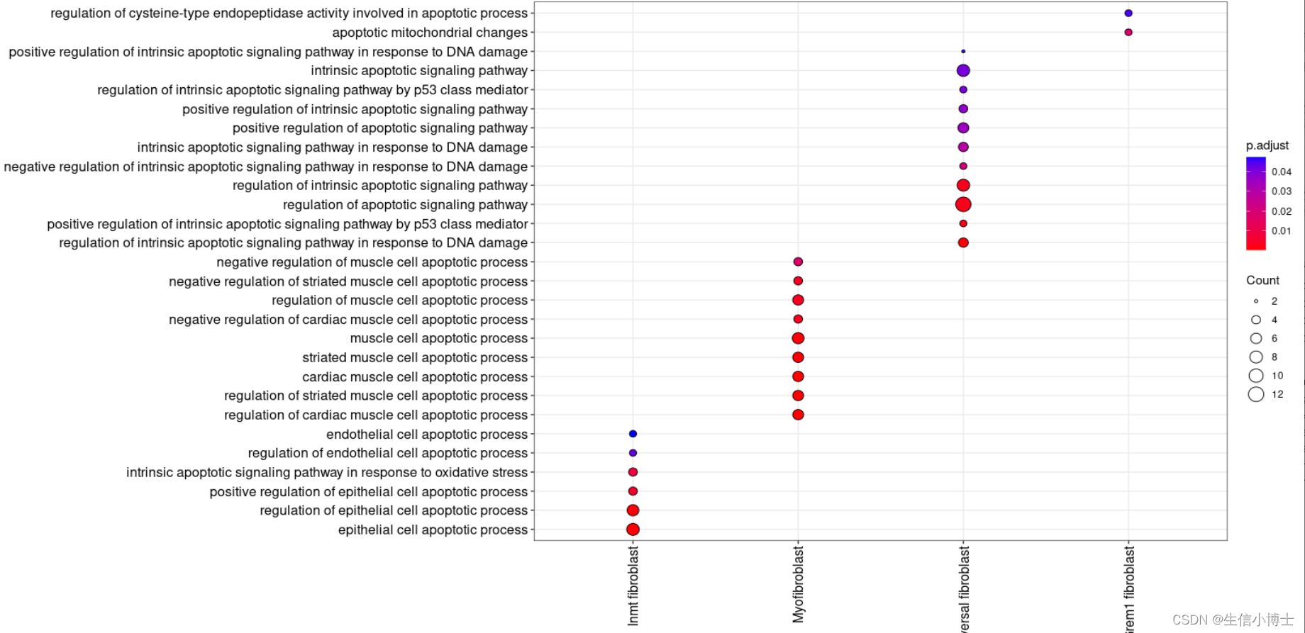
selected_clusterenrich=enrichmets[grepl(pattern = "lung alveolus developmen|extracellular matrix organization|extracellular structure organization|response to toxic substance|blood vessel endothelial cell migration
                                        regulation of blood vessel endothelial cell migration|lung development|respiratory tube development|detoxification|
                                        cellular response to toxic substance|endothelial cell proliferation|cellular response to chemical stress|
                                        Wnt|infla|fibrob|myeloid",
                                        x = enrichmets$Description) &
                                 stringr::str_detect(pattern = "muscle|fibroblast migration|positive regulation of endothelial cell proliferation|
                                                     inflammatory response to wounding|wound healing involved in inflammatory response|fibronectin binding|fibronectin binding|inflammatory response to wounding|fibronectin binding", negate = TRUE, string = enrichmets$Description)
                                    ,]

head(selected_clusterenrich) 

distinct(selected_clusterenrich)

# remove duplicate rows based on Description 并且保留其他所有变量
distinct_df <- distinct(selected_clusterenrich, Description,.keep_all = TRUE)

ggplot( distinct(selected_clusterenrich,Description,.keep_all=TRUE)  %>% 
          
          #  dplyr::mutate(Cluster = factor(Cluster, levels = unique(.$Cluster))) %>%
          
          dplyr::mutate(Description = factor(Description, levels = unique(.$Description))) %>%
          #  dplyr::group_by(Cluster)  %>%
         
          dplyr::filter(stringr::str_detect(pattern = "muscle", negate = TRUE,Description))  %>%
        
            add_count()  %>%
          dplyr::arrange(dplyr::desc(n),dplyr::desc(Description))  %>%
          mutate(Description =forcats:: fct_inorder(Description))
        
        , #fibri|matrix|colla
        aes(Cluster, y = Description)) +  #stringr:: str_wrap
  scale_y_discrete(labels = function(x) stringr::str_wrap(x, width = 58)) +  #调整terms长度 字符太长
  geom_point(aes(fill=p.adjust, size=Count), shape=21)+
  theme_bw()+
  theme(axis.text.x=element_text(angle=90,hjust = 1,vjust=0.5),
        axis.text.y=element_text(size = 12),
        axis.text = element_text(color = 'black', size = 12)
  )+
  scale_fill_gradient(low="red",high="blue")+
  labs(x=NULL,y=NULL)
# coord_flip()
print(getwd())