【Two Stream Net】

一，双语翻译

Abstract

We investigate architectures of discriminatively trained deep Convolutional Networks (ConvNets) for action recognition in video. The challenge is to capture the complementary information on appearance from still frames and motion between frames. We also aim to generalise the best performing hand-crafted features within a data-driven learning framework. Our contribution is three-fold. First, we propose a two-stream ConvNet architecture which incorporates spatial and temporal networks. Second, we demonstrate that a ConvNet trained on multi-frame dense optical flow is able to achieve very good performance in spite of limited training data. Finally, we show that multitask learning, applied to two different action classification datasets, can be used to increase the amount of training data and improve the performance on both. Our architecture is trained and evaluated on the standard video actions benchmarks of UCF-101 and HMDB-51, where it is competitive with the state of the art. It also exceeds by a large margin previous attempts to use deep nets for video classification

我们研究了用于视频动作识别的判别训练深度卷积网络（ConvNets）的体系结构。挑战在于从静止帧和帧之间的运动捕获关于外观的补充信息。我们还致力于在数据驱动的学习框架内推广性能最佳的手工制作功能。我们的贡献是三倍的。首先，我们提出了一种包含空间和时间网络的双流ConvNet架构。其次，我们证明了在多帧密集光流上训练的ConvNet能够在训练数据有限的情况下获得非常好的性能。最后，我们证明了应用于两个不同动作分类数据集的多任务学习可以用来增加训练数据量并提高两者的性能。我们的架构是在UCF-101和HMDB-51的标准视频动作基准上进行训练和评估的，在这些基准上它与最先进的技术相竞争。它还大大超过了以前使用深度网络进行视频分类的尝试。

1 Introduction

Recognition of human actions in videos is a challenging task which has received a significant amount of attention in the research community [11, 14, 17, 26]. Compared to still image classification, the temporal component of videos provides an additional (and important) clue for recognition, as a number of actions can be reliably recognised based on the motion information. Additionally, video provides natural data augmentation (jittering) for single image (video frame) classification.

识别视频中的人类行为是一项具有挑战性的任务，在研究界受到了大量关注[11，14，17，26]。与静态图像分类相比，视频的时间分量为识别提供了额外的（也是重要的）线索，因为可以基于运动信息可靠地识别许多动作。此外，视频为单个图像（视频帧）分类提供了自然的数据增强（抖动）

In this work, we aim at extending deep Convolutional Networks (ConvNets) [19], a state-of-theart still image representation [15], to action recognition in video data. This task has recently been addressed in [14] by using stacked video frames as input to the network, but the results were significantly worse than those of the best hand-crafted shallow representations [20, 26]. We investigate a different architecture based on two separate recognition streams (spatial and temporal), which are then combined by late fusion. The spatial stream performs action recognition from still video frames, whilst the temporal stream is trained to recognise action from motion in the form of dense optical flow. Both streams are implemented as ConvNets. Decoupling the spatial and temporal nets also allows us to exploit the availability of large amounts of annotated image data by pre-training the spatial net on the ImageNet challenge dataset [1]. Our proposed architecture is related to the two-streams hypothesis [9], according to which the human visual cortex contains two pathways: the ventral stream (which performs object recognition) and the dorsal stream (which recognises motion); though we do not investigate this connection any further here.

在这项工作中，我们的目标是将深度卷积网络（ConvNets）[19]（一种最先进的静态图像表示[15]）扩展到视频数据中的动作识别。这项任务最近在[14]中通过使用堆叠的视频帧作为网络输入来解决，但结果明显比最好的手工制作的浅层表示[20，26]差。我们研究了一种基于两个独立的识别流（空间和时间）的不同架构，然后通过后期融合将其组合在一起。空间流从静止视频帧中执行动作识别，而时间流被训练以从密集光流形式的运动中识别动作。这两个流都被实现为ConvNets。将空间和时间网络解耦还允许我们通过在ImageNet挑战数据集上预训练空间网络来利用大量注释图像数据的可用性[1]。我们提出的架构与双流假说[9]有关，根据该假说，人类视觉皮层包含两条通路：腹流（进行物体识别）和背流（识别运动）；尽管我们在这里不再进一步研究这种联系。

The rest of the paper is organised as follows. In Sect. 1.1 we review the related work on action recognition using both shallow and deep architectures. In Sect. 2 we introduce the two-stream architecture and specify the Spatial ConvNet. Sect. 3 introduces the Temporal ConvNet and in particular how it generalizes the previous architectures reviewed in Sect. 1.1. A mult-task learning framework is developed in Sect. 4 in order to allow effortless combination of training data over
multiple datasets. Implementation details are given in Sect. 5, and the performance is evaluated in Sect. 6 and compared to the state of the art. Our experiments on two challenging datasets (UCF- 101 [24] and HMDB-51 [16]) show that the two recognition streams are complementary, and our deep architecture significantly outperforms that of [14] and is competitive with the state of the artshallow representations [20, 21, 26] in spite of being trained on relatively small datasets.

论文的其余部分组织如下。在教派。1.1我们回顾了使用浅层和深层架构进行动作识别的相关工作。在教派。2我们介绍了双流结构，并指定了空间ConvNet。门派3介绍了时态ConvNet，特别是它如何概括第节中回顾的先前架构。1.1.在第节中开发了一个多任务学习框架。4以便在2014年11月12日的多个数据集上轻松组合训练数据。第节给出了实施细节。5，性能在第。6，并与现有技术进行了比较。我们在两个具有挑战性的数据集（UCF-101[24]和HMDB-51[16]）上的实验表明，这两个识别流是互补的，我们的深度架构显著优于[14]的深度架构，尽管在相对较小的数据集上进行了训练，但与现有技术的浅层表示[20，21，26]相比具有竞争力。

1.1 Related work

Video recognition research has been largely driven by the advances in image recognition methods, which were often adapted and extended to deal with video data. A large family of video action recognition methods is based on shallow high-dimensional encodings of local spatio-temporal features. For instance, the algorithm of [17] consists in detecting sparse spatio-temporal interest points,
which are then described using local spatio-temporal features: Histogram of Oriented Gradients (HOG) [7] and Histogram of Optical Flow (HOF). The features are then encoded into the Bag Of Features (BoF) representation, which is pooled over several spatio-temporal grids (similarly to spatial pyramid pooling) and combined with an SVM classifier. In a later work [28], it was shown that
dense sampling of local features outperforms sparse interest points.

视频识别研究在很大程度上是由图像识别方法的进步推动的，这些方法通常被调整和扩展以处理视频数据。一大类视频动作识别方法是基于局部时空特征的浅高维编码。例如，[17]的算法包括检测稀疏的时空兴趣点，然后使用局部时空特征来描述这些兴趣点：定向梯度直方图（HOG）[7]和光流直方图（HOF）。然后，将特征编码到特征袋（BoF）表示中，该特征袋在几个时空网格上进行合并（类似于空间金字塔合并），并与SVM分类器相结合。在后来的工作[28]中，表明局部特征的密集采样优于稀疏兴趣点。

Instead of computing local video features over spatio-temporal cuboids, state-of-the-art shallow video representations [20, 21, 26] make use of dense point trajectories. The approach, first introduced in [29], consists in adjusting local descriptor support regions, so that they follow dense trajectories, computed using optical flow. The best performance in the trajectory-based pipeline
was achieved by the Motion Boundary Histogram (MBH) [8], which is a gradient-based feature, separately computed on the horizontal and vertical components of optical flow. A combination of several features was shown to further boost the accuracy. Recent improvements of trajectory-base hand-crafted representations include compensation of global (camera) motion [10, 16, 26], and the use of the Fisher vector encoding [22] (in [26]) or its deeper variant [23] (in [21]).

最先进的浅层视频表示[20，21，26]利用密集点轨迹，而不是在时空长方体上计算局部视频特征。该方法首次在[29]中引入，包括调整局部描述符支持区域，使其遵循使用光流计算的密集轨迹。基于轨迹的管道中的最佳性能是通过运动边界直方图（MBH）[8]实现的，这是一种基于梯度的特征，分别根据光流的水平和垂直分量计算。几个特征的组合被证明可以进一步提高准确性。最近对基于轨迹的手工表示的改进包括全局（相机）运动的补偿[10，16，26]，以及使用Fisher矢量编码[22]（在[26]中）或其更深层次的变体[23]（在[21]中）。

There has also been a number of attempts to develop a deep architecture for video recognition. In the majority of these works, the input to the network is a stack of consecutive video frames, so the model is expected to implicitly learn spatio-temporal motion-dependent features in the first layers, which can be a difficult task. In [11], an HMAX architecture for video recognition was proposed
with pre-defined spatio-temporal filters in the first layer. Later, it was combined [16] with a spatial HMAX model, thus forming spatial (ventral-like) and temporal (dorsal-like) recognition streams. Unlike our work, however, the streams were implemented as hand-crafted and rather shallow (3- layer) HMAX models. In [4, 18, 25], a convolutional RBM and ISA were used for unsupervised learning of spatio-temporal features, which were then plugged into a discriminative model for action classification. Discriminative end-to-end learning of video ConvNets has been addressed in [12] and, more recently, in [14], who compared several ConvNet architectures for action recognition. Training was carried out on a very large Sports-1M dataset, comprising 1.1M YouTube videos of sports activities. Interestingly, [14] found that a network, operating on individual video frames,
performs similarly to the networks, whose input is a stack of frames. This might indicate that the learnt spatio-temporal features do not capture the motion well. The learnt representation, finetuned on the UCF-101 dataset, turned out to be 20% less accurate than hand-crafted state-of-the-art
trajectory-based representation [20, 27].

也有许多尝试开发用于视频识别的深层架构。在大多数这些工作中，网络的输入是一堆连续的视频帧，因此该模型有望隐含地学习第一层中的时空运动相关特征，这可能是一项艰巨的任务。在[11]中，提出了一种用于视频识别的HMAX架构，该架构在第一层中具有预定义的时空滤波器。后来，它与空间HMAX模型相结合[16]，从而形成了空间（腹侧样）和时间（背侧样）识别流。然而，与我们的工作不同的是，流被实现为手工制作的、相当浅的（3层）HMAX模型。在[4，18，25]中，卷积RBM和ISA用于时空特征的无监督学习，然后将其插入动作分类的判别模型中。[12]和最近的[14]中已经讨论了视频ConvNet的判别式端到端学习，他们比较了几种用于动作识别的ConvNet架构。训练是在一个非常大的Sports-1M数据集上进行的，该数据集包括110万个YouTube体育活动视频。有趣的是，[14]发现，对单个视频帧进行操作的网络的性能与网络类似，网络的输入是帧堆栈。这可能表明所学习的时空特征不能很好地捕捉运动。在UCF-101数据集上微调的学习表示比手工制作的最先进的基于轨迹的表示准确率低20%[20，27]。

Our temporal stream ConvNet operates on multiple-frame dense optical flow, which is typically computed in an energy minimisation framework by solving for a displacement field (typically at multiple image scales). We used a popular method of [2], which formulates the energy based on constancy assumptions for intensity and its gradient, as well as smoothness of the displacement field.
Recently, [30] proposed an image patch matching scheme, which is reminiscent of deep ConvNets, but does not incorporate learning.

我们的时间流ConvNet在多帧密集光流上运行，通常在能量最小化框架中通过求解位移场（通常在多个图像尺度上）来计算。我们使用了[2]的一种流行方法，该方法基于强度及其梯度的恒定性假设以及位移场的光滑性来公式化能量。最近，[30]提出了一种图像补丁匹配方案，它让人想起深度ConvNets，但不包含学习。

2 Two-stream architecture for video recognition

Video can naturally be decomposed into spatial and temporal components. The spatial part, in the form of individual frame appearance, carries information about scenes and objects depicted in the video. The temporal part, in the form of motion across the frames, conveys the movement of the observer (the camera) and the objects. We devise our video recognition architecture accordingly,
dividing it into two streams, as shown in Fig. 1. Each stream is implemented using a deep ConvNet, softmax scores of which are combined by late fusion. We consider two fusion methods: averaging and training a multi-class linear SVM [6] on stacked L2-normalised softmax scores as features.

视频可以自然地分解为空间和时间分量。空间部分以单独的帧外观的形式携带关于视频中描绘的场景和对象的信息。时间部分，以跨帧运动的形式，传达观察者（相机）和物体的运动。我们相应地设计了我们的视频识别架构，将其分为两个流，如图1所示。每个流都使用深度ConvNet来实现，其softmax分数通过后期融合来组合。我们考虑两种融合方法：在堆叠的L2归一化softmax分数上平均和训练多类线性SVM[6]作为特征。

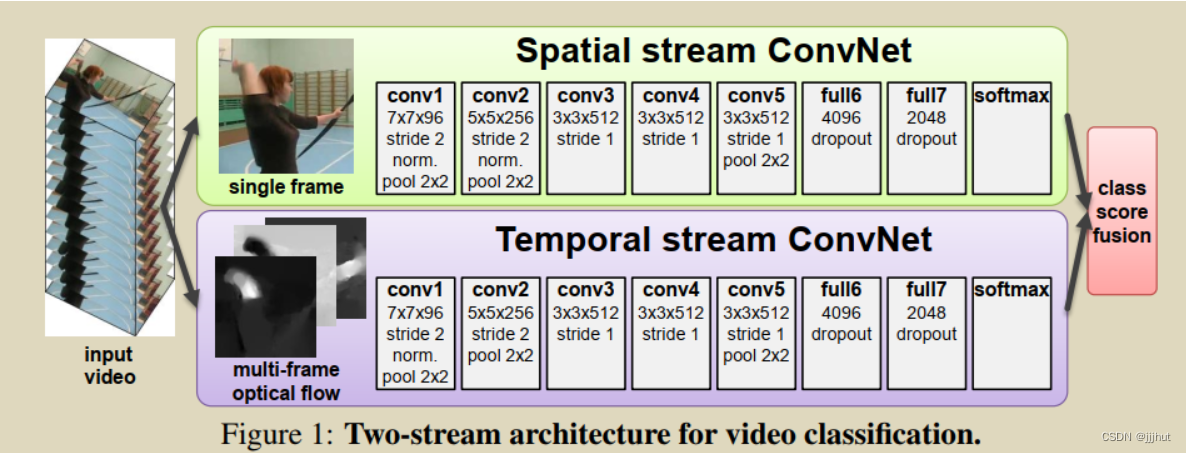
Spatial stream ConvNet operates on individual video frames, effectively performing action recognition from still images. The static appearance by itself is a useful clue, since some actions are strongly associated with particular objects. In fact, as will be shown in Sect. 6, action classification from still frames (the spatial recognition stream) is fairly competitive on its own. Since a spatial
ConvNet is essentially an image classification architecture, we can build upon the recent advances in large-scale image recognition methods [15], and pre-train the network on a large image classification dataset, such as the ImageNet challenge dataset. The details are presented in Sect. 5. Next, we describe the temporal stream ConvNet, which exploits motion and significantly improves accuracy.

空间流ConvNet对单个视频帧进行操作，有效地从静止图像中执行动作识别。静态外观本身就是一条有用的线索，因为有些动作与特定对象有很强的关联。事实上，正如第三节所示。6，来自静止帧（空间识别流）的动作分类本身就相当有竞争力。由于空间ConvNet本质上是一种图像分类架构，我们可以在大规模图像识别方法[15]的最新进展的基础上，在大型图像分类数据集（如ImageNet挑战数据集）上预训练网络。细节见第节。5.接下来，我们描述了时间流ConvNet，它利用了运动并显著提高了精度。

3 Optical flow ConvNets

In this section, we describe a ConvNet model, which forms the temporal recognition stream of our architecture (Sect. 2). Unlike the ConvNet models, reviewed in Sect. 1.1, the input to our model is formed by stacking optical flow displacement fields between several consecutive frames. Such input
explicitly describes the motion between video frames, which makes the recognition easier, as the network does not need to estimate motion implicitly. We consider several variations of the optical
flow-based input, which we describe below.

在本节中，我们描述了一个ConvNet模型，它形成了我们架构的时间识别流（Sect.2）。与ConvNet模型不同，第。1.1，我们的模型的输入是通过在几个连续帧之间堆叠光流位移场而形成的。这样的输入明确地描述了视频帧之间的运动，这使得识别更容易，因为网络不需要隐含地估计运动。我们考虑基于光流的输入的几种变体，我们将在下面进行描述。

Figure 2: Optical flow. (a),(b): a pair of consecutive video frames with the area around a moving hand outlined with a cyan rectangle. ©: a close-up of dense optical flow in the outlined area; (d): horizontal component dx of the displacement vector field (higher intensity corresponds to positive values, lower intensity to negative values). (e): vertical component dy. Note how (d) and (e) highlight the moving hand and bow. The input to a ConvNet contains multiple flows (Sect. 3.1).

图2：光流。（a） ，（b）：一对连续的视频帧，移动的手周围的区域用青色矩形勾勒。（c） ：轮廓区域内密集光流的特写；（d） ：位移矢量场的水平分量dx（强度越高对应正值，强度越低对应负值）。（e） ：垂直分量dy.注意（d）和（e）如何突出显示移动的手和弓。ConvNet的输入包含多个流（第3.1节）。

3.1 ConvNet input configurations

Optical flow stacking. A dense optical flow can be seen as a set of displacement vector fields dt between the pairs of consecutive frames t and t + 1. By dt(u; v) we denote the displacement vector at the point (u; v) in frame t, which moves the point to the corresponding point in the following frame t + 1. The horizontal and vertical components of the vector field, dx t and dy t , can be seen as image channels (shown in Fig. 2), well suited to recognition using a convolutional network. To represent the motion across a sequence of frames, we stack the flow channels dx;y t of L consecutive frames to form a total of 2L input channels. More formally, let w and h be the width and height of a video; a ConvNet input volume Iτ 2 Rw×h×2L for an arbitrary frame τ is then constructed as follows:

光流堆叠。密集的光流可以看作是连续帧对t和t+1之间的一组位移矢量场dt。通过dt（u；v），我们表示在帧t中的点（u；v）处的位移矢量，该位移矢量将该点移动到下一帧t+1中的对应点。矢量场的水平和垂直分量dx t和dy t可以被视为图像通道（如图所示）。2）非常适合使用卷积网络进行识别。为了表示跨帧序列的运动，我们堆叠流动通道dx；y t，以形成总共2L个输入通道。更正式地说，让w和h是视频的宽度和高度；任意帧τ的ConvNet输入体积Iτ2Rw×h×2L构造如下：

where pk is the k-th point along the trajectory, which starts at the location (u; v) in the frame τ and is defined by the following recurrence relation:

其中pk是沿轨迹的第k个点，该点从帧τ中的位置（u；v）开始，由以下递推关系定义：

Compared to the input volume representation (1), where the channels Iτ (u; v; c) store the displacement vectors at the locations (u; v), the input volume (2) stores the vectors sampled at the locations pk along the trajectory (as illustrated in Fig. 3-right).

与输入体积表示（1）相比，其中通道Iτ（u；v；c）存储位置（u；v）处的位移矢量，输入体积（2）存储沿轨迹在位置pk处采样的矢量（如图3所示，右侧）。

Figure 3: ConvNet input derivation from the multi-frame optical flow. Left: optical flow stacking (1) samples the displacement vectors d at the same location in multiple frames. Right: trajectory stacking (2) samples the vectors along the trajectory. The frames and the corresponding displacement vectors are shown with the same colour.

图3：来自多帧光流的ConvNet输入推导。左图：光流叠加（1）对多帧中相同位置的位移矢量d进行采样。右图：轨迹堆叠（2）沿轨迹对向量进行采样。帧和相应的位移矢量以相同的颜色显示。

Bi-directional optical flow. Optical flow representations (1) and (2) deal with the forward optical flow, i.e. the displacement field dt of the frame t specifies the location of its pixels in the following frame t + 1. It is natural to consider an extension to a bi-directional optical flow, which can be obtained by computing an additional set of displacement fields in the opposite direction. We then construct an input volume Iτ by stacking L=2 forward flows between frames τ and τ +L=2 and L=2 backward flows between frames τ - L=2 and τ. The input Iτ thus has the same number of channels (2L) as before. The flows can be represented using either of the two methods (1) and (2).

双向光流。光流表示（1）和（2）处理正向光流，即帧t的位移场dt指定其像素在下一帧t+1中的位置。考虑双向光流的扩展是很自然的，这可以通过计算相反方向上的一组额外的位移场来获得。然后，我们通过堆叠帧τ和τ之间的L=2个正向流+帧τ−L=2和τ之间L=2个反向流来构造输入体积Iτ。因此，输入Iτ具有与以前相同数量的通道（2L）。可以使用两种方法（1）和（2）中的任一种来表示流。

Mean flow subtraction. It is generally beneficial to perform zero-centering of the network input, as it allows the model to better exploit the rectification non-linearities. In our case, the displacement vector field components can take on both positive and negative values, and are naturally centered in the sense that across a large variety of motions, the movement in one direction is as probable as the movement in the opposite one. However, given a pair of frames, the optical flow between them can be dominated by a particular displacement, e.g. caused by the camera movement. The importance of camera motion compensation has been previously highlighted in [10, 26], where a global motion component was estimated and subtracted from the dense flow. In our case, we consider a simpler approach: from each displacement field d we subtract its mean vector.

平均流量减法。执行网络输入的零居中通常是有益的，因为它允许模型更好地利用整流非线性。在我们的情况下，位移矢量场分量可以取正值和负值，并且自然地集中在这样一种意义上，即在各种各样的运动中，一个方向上的运动与相反方向上的移动一样可能。然而，给定一对帧，它们之间的光流可以由特定的位移主导，例如由相机移动引起的位移。相机运动补偿的重要性在[10，26]中已经强调过，其中估计了全局运动分量并从稠密流中减去。在我们的例子中，我们考虑一种更简单的方法：从每个位移场d中减去其平均向量。

Architecture. Above we have described different ways of combining multiple optical flow displacement fields into a single volume Iτ 2 Rw×h×2L. Considering that a ConvNet requires a fixed-size input, we sample a 224 × 224 × 2L sub-volume from Iτ and pass it to the net as input. The hidden layers configuration remains largely the same as that used in the spatial net, and is illustrate in Fig. 1. Testing is similar to the spatial ConvNet, and is described in detail in Sect. 5.

建筑学上面我们描述了将多个光流位移场组合成单个体积Iτ2Rw×h×2L的不同方法。考虑到ConvNet需要固定大小的输入，我们从Iτ中采样224×224×2L子体积，并将其作为输入传递到网络。隐藏层配置与空间网络中使用的配置基本相同，如图所示。1。测试类似于空间ConvNet，并在第。5.

3.2 Relation of the temporal ConvNet architecture to previous representations

In this section, we put our temporal ConvNet architecture in the context of prior art, drawing connections to the video representations, reviewed in Sect. 1.1. Methods based on feature encodings [17, 29] typically combine several spatio-temporal local features. Such features are computed from the optical flow and are thus generalised by our temporal ConvNet. Indeed, the HOF and MBH local descriptors are based on the histograms of orientations of optical flow or its gradient, which can be obtained from the displacement field input (1) using a single convolutional layer (containing orientation-sensitive filters), followed by the rectification and pooling layers. The kinematic features of [10] (divergence, curl and shear) are also computed from the optical flow gradient, and, again, can
be captured by our convolutional model. Finally, the trajectory feature [29] is computed by stacking the displacement vectors along the trajectory, which corresponds to the trajectory stacking (2). In Sect. 3.3 we visualise the convolutional filters, learnt in the first layer of the temporal network. This provides further evidence that our representation generalises hand-crafted features.

在本节中，我们将我们的时态ConvNet架构放在现有技术的背景下，绘制与视频表示的连接，如第节所述。1.1.基于特征编码的方法[17，29]通常结合几个时空局部特征。这些特征是从光流中计算出来的，因此通过我们的时间ConvNet进行了推广。事实上，HOF和MBH4局部描述符是基于光流的方向或其梯度的直方图，其可以使用单个卷积层（包含方向敏感滤波器）从位移场输入（1）获得，然后是整流和池化层。[10]的运动学特征（发散、卷曲和剪切）也根据光流梯度计算，并且可以再次通过我们的卷积模型来捕捉。最后，通过沿轨迹叠加位移矢量来计算轨迹特征[29]，这对应于轨迹叠加（2）。在教派。3.3我们将在时间网络的第一层中学习的卷积滤波器可视化。这提供了进一步的证据，证明我们的表示概括了手工制作的功能。

As far as the deep networks are concerned, a two-stream video classification architecture of [16]
contains two HMAX models which are hand-crafted and less deep than our discriminatively trained
ConvNets, which can be seen as a learnable generalisation of HMAX. The convolutional models
of [12, 14] do not decouple spatial and temporal recognition streams, and rely on the motionsensitive convolutional filters, learnt from the data. In our case, motion is explicitly represented
using the optical flow displacement field, computed based on the assumptions of constancy of the
intensity and smoothness of the flow. Incorporating such assumptions into a ConvNet framework
might be able to boost the performance of end-to-end ConvNet-based methods, and is an interesting
direction for future research.

就深度网络而言，[16]的双流视频分类体系结构包含两个手工制作的HMAX模型，其深度不如我们经过区别训练的ConvNets，这可以被视为HMAX的可学习概括。[12，14]的卷积模型不解耦空间和时间识别流，而是依赖于从数据中学习的运动敏感卷积滤波器。在我们的情况下，运动是使用光流位移场来明确表示的，该场是基于流的强度和平滑度的恒定性假设来计算的。将这些假设纳入ConvNet框架可能能够提高基于端到端ConvNet的方法的性能，这是未来研究的一个有趣方向。

Figure 4: First-layer convolutional filters learnt on 10 stacked optical flows. The visualisation
is split into 96 columns and 20 rows: each column corresponds to a filter, each row – to an input
channel.

图4：在10个堆叠光流上学习的第一层卷积滤波器。可视化分为96列和20行：每列对应一个过滤器，每行对应一个输入通道。

In Fig. 4 we visualise the convolutional filters from the first layer of the temporal ConvNet, trained
on the UCF-101 dataset. Each of the 96 filters has a spatial receptive field of 7 × 7 pixels, and spans
20 input channels, corresponding to the horizontal (dx) and vertical (dy) components of 10 stacked
optical flow displacement fields d.

在图4中，我们可视化了在UCF-101数据集上训练的时间ConvNet第一层的卷积滤波器。96个滤波器中的每个滤波器具有7×7像素的空间感受野，并且跨越20个输入通道，对应于10个堆叠的光流位移场d的水平（dx）和垂直（dy）分量。

As can be seen, some filters compute spatial derivatives of the optical flow, capturing how motion changes with image location, which generalises derivative-based hand-crafted descriptors (e.g.
MBH). Other filters compute temporal derivatives, capturing changes in motion over time.

可以看出，一些滤波器计算光流的空间导数，捕捉运动如何随图像位置而变化，这概括了基于导数的手工描述符（例如MBH）。其他滤波器计算时间导数，捕捉运动随时间的变化。

4 Multi-task learning

Unlike the spatial stream ConvNet, which can be pre-trained on a large still image classification dataset (such as ImageNet), the temporal ConvNet needs to be trained on video data – and the available datasets for video action classification are still rather small. In our experiments (Sect. 6), training is performed on the UCF-101 and HMDB-51 datasets, which have only: 9.5K and 3.7K videos respectively. To decrease over-fitting, one could consider combining the two datasets into one; this, however, is not straightforward due to the intersection between the sets of classes. One option (which we evaluate later) is to only add the images from the classes, which do not appear in the original dataset. This, however, requires manual search for such classes and limits the amount of additional training data.

与可以在大型静态图像分类数据集（如ImageNet）上预训练的空间流ConvNet不同，时间ConvNet需要在视频数据上进行训练，并且用于视频动作分类的可用数据集仍然相当小。在我们的实验中（第6节），在UCF-101和HMDB-51数据集上进行训练，这两个数据集分别只有：9.5K和3.7K的视频。为了减少过度拟合，可以考虑将两个数据集合并为一个数据集；然而，由于类集合之间的交集，这并不简单。一种选择（我们稍后评估）是只添加类中的图像，这些图像不会出现在原始数据集中。然而，这需要手动搜索此类类，并限制了额外训练数据的数量。

A more principled way of combining several datasets is based on multi-task learning [5]. Its aim is to learn a (video) representation, which is applicable not only to the task in question (such as HMDB-51 classification), but also to other tasks (e.g. UCF-101 classification). Additional tasks act as a regulariser, and allow for the exploitation of additional training data. In our case, a ConvNet architecture is modified so that it has two softmax classification layers on top of the last fully- connected layer: one softmax layer computes HMDB-51 classification scores, the other one – the UCF-101 scores. Each of the layers is equipped with its own loss function, which operates only on the videos, coming from the respective dataset. The overall training loss is computed as the sum of the individual tasks’ losses, and the network weight derivatives can be found by back-propagation.

一种更有原则的组合多个数据集的方法是基于多任务学习[5]。其目的是学习（视频）表示，该表示不仅适用于所讨论的任务（如HMDB-51分类），还适用于其他任务（如UCF-101分类）。额外的任务充当规则器，并允许利用额外的训练数据。在我们的案例中，对ConvNet架构进行了修改，使其在最后一个完全连接的层之上有两个softmax分类层：一个softmax层计算HMDB-51分类分数，另一个计算UCF-101分数。每个层都配备了自己的损失函数，该函数仅对来自相应数据集的视频进行操作。总训练损失计算为单个任务损失的总和，网络权重导数可以通过反向传播找到。

5 Implementation details

ConvNets configuration. The layer configuration of our spatial and temporal ConvNets is schematically shown in Fig. 1. It corresponds to CNN-M-2048 architecture of [3] and is similar to the network of [31]. All hidden weight layers use the rectification (ReLU) activation function; maxpooling is performed over 3×3 spatial windows with stride 2; local response normalisation uses the same settings as [15]. The only difference between spatial and temporal ConvNet configurations is that we removed the second normalisation layer from the latter to reduce memory consumption.

ConvNets配置。我们的空间和时间卷积网的层配置如图1所示。它对应于[3]的CNN-M-2048架构，类似于[31]的网络。所有隐藏权重层都使用整流（ReLU）激活功能；以及maxpooling是在3×3个空间窗口上执行的，步长为2；局部响应规范化使用与[15]相同的设置。空间和时间ConvNet配置之间的唯一区别是，我们从后者中删除了第二个归一化层，以减少内存消耗。

Training. The training procedure can be seen as an adaptation of that of [15] to video frames, and is generally the same for both spatial and temporal nets. The network weights are learnt using the mini-batch stochastic gradient descent with momentum (set to 0.9). At each iteration, a mini-batch of 256 samples is constructed by sampling 256 training videos (uniformly across the classes), from each of which a single frame is randomly selected. In spatial net training, a 224 × 224 sub-image is randomly cropped from the selected frame; it then undergoes random horizontal flipping and RGB jittering. The videos are rescaled beforehand, so that the smallest side of the frame equals 256. We note that unlike [15], the sub-image is sampled from the whole frame, not just its 256 × 256 center. In the temporal net training, we compute an optical flow volume I for the selected training frame as described in Sect. 3. From that volume, a fixed-size 224 × 224 × 2L input is randomly cropped and flipped. The learning rate is initially set to 10-2, and then decreased according to a fixed schedule,which is kept the same for all training sets. Namely, when training a ConvNet from scratch, the rate is changed to 10-3 after 50K iterations, then to 10-4 after 70K iterations, and training is stopped
after 80K iterations. In the fine-tuning scenario, the rate is changed to 10-3 after 14K iterations, and training stopped after 20K iterations.

训练.训练过程可以被视为[15]对视频帧的适应，并且对于空间和时间网络通常是相同的。网络权重是使用具有动量的小批量随机梯度下降（设置为0.9）来学习的。在每次迭代中，通过对256个训练视频进行采样（均匀地跨类），构建一个由256个样本组成的小批量，从每个视频中随机选择一帧。在空间网训练中，从所选帧中随机裁剪224×224个子图像；然后它经历随机水平翻转和RGB抖动。视频被预先重新缩放，使得帧的最小边等于256。我们注意到，与[15]不同，子图像是从整个帧中采样的，而不仅仅是其256×256的中心。在时间网络训练中，我们计算所选训练帧的光流体积I，如第。3.从该体积中，随机裁剪和翻转固定大小的224×224×2L输入。学习率最初设置为10−2，然后根据固定的时间表降低，所有训练集都保持不变。也就是说，当从头开始训练ConvNet时，速率在50K迭代后更改为10−3，然后在70K迭代后改为10−4，并且在80K迭代后停止训练。在微调场景中，14K迭代后，速率更改为10−3，20K迭代后停止训练。

Testing. At test time, given a video, we sample a fixed number of frames (25 in our experiments) with equal temporal spacing between them. From each of the frames we then obtain 10 ConvNet inputs [15] by cropping and flipping four corners and the center of the frame. The class scores for the whole video are then obtained by averaging the scores across the sampled frames and crops therein.

测试。在测试时，给定一个视频，我们对固定数量的帧（实验中为25帧）进行采样，它们之间的时间间隔相等。然后，从每个帧中，我们通过裁剪和翻转帧的四个角和中心来获得10个ConvNet输入[15]。然后通过对采样的帧和其中的裁剪的得分进行平均来获得整个视频的类得分。

Pre-training on ImageNet ILSVRC-2012. When pre-training the spatial ConvNet, we use the same training and test data augmentation as described above (cropping, flipping, RGB jittering). This yields 13:5% top-5 error on ILSVRC-2012 validation set, which compares favourably to 16:0% reported in [31] for a similar network. We believe that the main reason for the improvement is sampling of ConvNet inputs from the whole image, rather than just its center.

在ImageNet ILSVRC-2012上预训练。在预训练spatial ConvNet时，我们使用与上述相同的训练和测试数据增强方法（裁剪、翻转、RGB抖动）。这在ILSVRC-2012验证集上产生了13:5%的前5个错误，与[31]中报告的类似网络的16:0%相比，这是有利的。我们认为，改进的主要原因是从整个图像中采样ConvNet输入，而不仅仅是它的中心。

Multi-GPU training. Our implementation is derived from the publicly available Caffe toolbox [13], but contains a number of significant modifications, including parallel training on multiple GPUs installed in a single system. We exploit the data parallelism, and split each SGD batch across several GPUs. Training a single temporal ConvNet takes 1 day on a system with 4 NVIDIA Titan cards, which constitutes a 3:2 times speed-up over single-GPU training.

多GPU训练。我们的实现源于公开可用的Caffe工具箱[13]，但包含许多重大修改，包括在单个系统中安装的多个GPU上进行并行训练。我们利用数据并行性，并将每个SGD批划分为几个GPU。在具有4个NVIDIA Titan卡的系统上训练单个时态ConvNet需要1天时间，这比单个GPU训练的速度提高了3:2倍。

Optical flow is computed using the off-the-shelf GPU implementation of [2] from the OpenCV
toolbox. In spite of the fast computation time (0:06s for a pair of frames), it would still introduce
a bottleneck if done on-the-fly, so we pre-computed the flow before training. To avoid storing
the displacement fields as floats, the horizontal and vertical components of the flow were linearly
rescaled to a [0; 255] range and compressed using JPEG (after decompression, the flow is rescaled back to its original range). This reduced the flow size for the UCF-101 dataset from 1.5TB to 27GB.

光流是使用OpenCV工具箱中[2]的现成GPU实现来计算的。尽管计算时间很快（一对帧为0:06s），但如果在飞行中完成，仍然会引入瓶颈，因此我们在训练前预先计算了流量。为了避免将位移场存储为浮动，将流的水平和垂直分量线性地重新缩放到[0；255]范围，并使用JPEG压缩（解压缩后，流将重新缩放回其原始范围）。这将UCF-101数据集的流量大小从1.5TB减少到27GB。

6 Evaluation

Datasets and evaluation protocol. The evaluation is performed on UCF-101 [24] and HMDB-51 [16] action recognition benchmarks, which are among the largest available annotated video datasets1. UCF-101 contains 13K videos (180 frames/video on average), annotated into 101 action classes; HMDB-51 includes 6.8K videos of 51 actions. The evaluation protocol is the same for both datasets: the organisers provide three splits into training and test data, and the performance is measured by the mean classification accuracy across the splits. Each UCF-101 split contains 9.5K training videos; an HMDB-51 split contains 3.7K training videos. We begin by comparing different architectures on the first split of the UCF-101 dataset. For comparison with the state of the art, we follow the standard evaluation protocol and report the average accuracy over three splits on both UCF-101 and HMDB-51.

数据集和评估协议。评估是在UCF-101[24]和HMDB-51[16]动作识别基准上进行的，这两个基准是最大的可用注释视频数据集1。UCF-101包含13K视频（平均180帧/视频），注释为101个动作类；HMDB-51包括51个动作的6.8K视频。对于这两个数据集评估方案相同：组织者提供了三个分为训练和测试数据的数据集，其性能通过分为三个数据集的平均分类精度来衡量。每个UCF-101拆分包含9.5K训练视频；HMDB-51拆分版包含3.7K训练视频。我们首先在UCF-101数据集的第一部分上比较不同的体系结构。为了与现有技术进行比较，我们遵循标准评估协议，并报告了UCF-101和HMDB-51上三次拆分的平均准确度。

Spatial ConvNets. First, we measure the performance of the spatial stream ConvNet. Three scenarios are considered: (i) training from scratch on UCF-101, (ii) pre-training on ILSVRC-2012
followed by fine-tuning on UCF-101, (iii) keeping the pre-trained network fixed and only training
the last (classification) layer. For each of the settings, we experiment with setting the dropout regularisation ratio to 0:5 or to 0:9. From the results, presented in Table 1a, it is clear that training the ConvNet solely on the UCF-101 dataset leads to over-fitting (even with high dropout), and is inferior to pre-training on a large ILSVRC-2012 dataset. Interestingly, fine-tuning the whole network gives only marginal improvement over training the last layer only. In the latter setting, higher dropout over-regularises learning and leads to worse accuracy. In the following experiments we opted for training the last layer on top of a pre-trained ConvNet.

空间 ConvNets。首先，我们测量了空间流ConvNet的性能。考虑了三种场景：（i）在UCF-101上从头开始训练，（ii）在ILSVRC-2012上进行预训练，然后在UCF-1101上进行微调，（iii）保持预训练的网络固定，只训练最后一层（分类）。对于每种设置，我们都将脱落正则化比率设置为0:5或0:9。从表1a中给出的结果可以清楚地看出，仅在UCF-101数据集上训练ConvNet会导致过度拟合（即使是高丢弃），并且不如在大型ILSVRC-2012数据集上进行预训练。有趣的是，与只训练最后一层相比，对整个网络进行微调只会带来边际改进。在后一种情况下，辍学率越高，学习越规范，准确性越差。在下面的实验中，我们选择在预先训练的ConvNet上训练最后一层。

Temporal ConvNets. Having evaluated spatial ConvNet variants, we now turn to the temporal
ConvNet architectures, and assess the effect of the input configurations, described in Sect. 3.1. In particular, we measure the effect of: using multiple (L = f5; 10g) stacked optical flows; trajectory stacking; mean displacement subtraction; using the bi-directional optical flow. The architectures are trained on the UCF-101 dataset from scratch, so we used an aggressive dropout ratio of 0:9 to help improve generalisation. The results are shown in Table 1b. First, we can conclude that stacking multiple (L > 1) displacement fields in the input is highly beneficial, as it provides the network with long-term motion information, which is more discriminative than the flow between a pair of frames (L = 1 setting). Increasing the number of input flows from 5 to 10 leads to a smaller improvement, so we kept L fixed to 10 in the following experiments. Second, we find that mean subtraction is helpful, as it reduces the effect of global motion between the frames. We use it in the following experiments as default. The difference between different stacking techniques is marginal; it turns out that optical flow stacking performs better than trajectory stacking, and using the bi-directional optical flow is only slightly better than a uni-directional forward flow. Finally, we note that temporal ConvNets significantly outperform the spatial ConvNets (Table 1a), which confirms the importance of motion information for action recognition.

时间卷积。在评估了空间ConvNet变体后，我们现在转向时间ConvNet架构，并评估输入配置的影响，如第。3.1.特别地，我们测量了以下效应：使用多个（L=f5；10g）堆叠的光流；轨迹叠加；平均位移减法；使用双向光流。这些体系结构是在UCF-101数据集上从头开始训练的，因此我们使用0:9的主动丢弃率来帮助提高泛化能力。结果如表1b所示。首先，我们可以得出结论，在输入中叠加多个（L>1）位移场是非常有益的，因为它为网络提供了长期运动信息，这比一对帧之间的流（L=1设置）更有鉴别力。将输入流的数量从5增加到10会导致较小的改进，因此在下面的实验中，我们将L固定为10。其次，我们发现均值减法是有帮助的，因为它减少了帧之间全局运动的影响。我们在以下实验中使用它作为默认值。不同堆叠技术之间的差异很小；结果表明，光流叠加的性能优于轨迹叠加，而使用双向光流仅略好于单向正向流。最后，我们注意到时间卷积网显著优于空间卷积网（表1a），这证实了运动信息对动作识别的重要性。

We also implemented the “slow fusion” architecture of [14], which amounts to applying a ConvNet to a stack of RGB frames (11 frames in our case). When trained from scratch on UCF-101, it achieved 56:4% accuracy, which is better than a single-frame architecture trained from scratch (52:3%), but is still far off the network trained from scratch on optical flow. This shows that while multi-frame information is important, it is also important to present it to a ConvNet in an appropriate manner.

我们还实现了[14]的“慢融合”架构，相当于将ConvNet应用于RGB帧堆栈（在我们的情况下为11帧）。当在UCF-101上从头开始训练时，它实现了56:4%的准确率，这比从头开始训练的单帧架构（52:3%）要好，但与在光流上从头开始培训的网络相比仍有很大差距。这表明，虽然多帧信息很重要，但以适当的方式将其呈现给ConvNet也很重要。

Multi-task learning of temporal ConvNets. Training temporal ConvNets on UCF-101 is challenging due to the small size of the training set. An even bigger challenge is to train the ConvNet on HMDB-51, where each training split is 2:6 times smaller than that of UCF-101. Here we evaluate different options for increasing the effective training set size of HMDB-51: (i) fine-tuning a temporal network pre-trained on UCF-101; (ii) adding 78 classes from UCF-101, which are manually selected so that there is no intersection between these classes and the native HMDB-51 classes; (iii) using the multi-task formulation (Sect. 4) to learn a video representation, shared between the UCF-101 and HMDB-51 classification tasks. The results are reported in Table 2. As expected, it is beneficial to utilise full (all splits combined) UCF-101 data for training (either explicitly by borrowing images, or implicitly by pre-training). Multi-task learning performs the best, as it allows the training procedure to exploit all available training data.

时态卷积网络的多任务学习。由于训练集的规模较小，在UCF-101上训练临时ConvNets具有挑战性。一个更大的挑战是在HMDB-51上训练ConvNet，其中每个训练分割比UCF-101的训练分割小2-6倍。在这里，我们评估了增加HMDB-51的有效训练集大小的不同选项：（i）微调在UCF-101上预训练的时间网络；（ii）从UCF-101中添加78个类，这些类是手动选择的，使得这些类与原生HMDB-51类之间没有交集；（iii）使用多任务公式（Sect.4）来学习在UCF-101和HMDB-51分类任务之间共享的视频表示。结果见表2。正如预期，这有益于利用完整的（所有分割组合的）UCF-101数据进行训练（明确地通过借用图像，或隐含地通过预训练）。多任务学习表现最好，因为它允许训练过程利用所有可用的训练数据。

We have also experimented with multi-task learning on the UCF-101 dataset, by training a network to classify both the full HMDB-51 data (all splits combined) and the UCF-101 data (a single split). On the first split of UCF-101, the accuracy was measured to be 81.5%, which improves on 81:0% achieved using the same settings, but without the additional HMDB classification task (Table 1b).

我们还在UCF-101数据集上进行了多任务学习的实验，通过训练网络对完整的HMDB-51数据（所有拆分组合在一起）和UCF-101（单个拆分）进行分类。在UCF-101的第一次拆分中，测量到的准确率为81.5%，在使用相同设置但没有额外HMDB分类任务的情况下提高了81:0%（表1b）。

Two-stream ConvNets. Here we evaluate the complete two-stream model, which combines the two recognition streams. One way of combining the networks would be to train a joint stack of
fully-connected layers on top of full6 or full7 layers of the two nets. This, however, was not feasibl in our case due to over-fitting. We therefore fused the softmax scores using either averaging or
a linear SVM. From Table 3 we conclude that: (i) temporal and spatial recognition streams are
complementary, as their fusion significantly improves on both (6% over temporal and 14% over
spatial nets); (ii) SVM-based fusion of softmax scores outperforms fusion by averaging; (iii) using
bi-directional flow is not beneficial in the case of ConvNet fusion; (iv) temporal ConvNet, trained
using multi-task learning, performs the best both alone and when fused with a spatial net.

双流ConvNets。在这里，我们评估了完整的双流模型，该模型结合了两个识别流。组合网络的一种方式是在两个网络的full6或full7层之上训练完全连接层的联合堆栈。然而，在我们的案例中，由于过度拟合，这是不可行的。因此，我们使用平均或线性SVM来融合softmax分数。从表3中，我们得出结论：（i）时间和空间识别流是互补的，因为它们的融合在两者上都有显著改善（在时间网络上为6%，在空间网络上为14%）；（ii）基于SVM的softmax分数的融合通过平均优于融合；（iii）在ConvNet融合的情况下，使用双向流是不利的；（iv）使用多任务学习训练的时态ConvNet，无论是单独还是与空间网络融合时都表现最好。

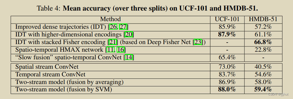
Comparison with the state of the art. We conclude the experimental evaluation with the comparison against the state of the art on three splits of UCF-101 and HMDB-51. For that we used a spatial net, pre-trained on ILSVRC, with the last layer trained on UCF or HMDB. The temporal net was trained on UCF and HMDB using multi-task learning, and the input was computed using uni-directional optical flow stacking with mean subtraction. The softmax scores of the two nets were combined using averaging or SVM. As can be seen from Table 4, both our spatial and temporal nets alone outperform the deep architectures of [14, 16] by a large margin. The combination of the two nets further improves the results (in line with the single-split experiments above), and is comparable to the very recent state-of-the-art hand-crafted models [20, 21, 26].

与现有技术的比较。我们通过对UCF-101和HMDB-51的三种拆分进行与现有技术比较来总结实验评估。为此，我们使用了一个空间网，在ILSVRC上进行预训练，最后一层在UCF或HMDB上进行训练。使用多任务学习在UCF和HMDB上训练时间网络，并使用带有平均减法的单向光流叠加来计算输入。使用平均或SVM将两个网络的softmax得分进行组合。从表4中可以看出，仅我们的空间和时间网络就在很大程度上优于[14，16]的深度架构。两种网络的组合进一步改善了结果（与上述单次分割实验一致），并与最新的最先进的手工制作模型相媲美[20，21，26]。

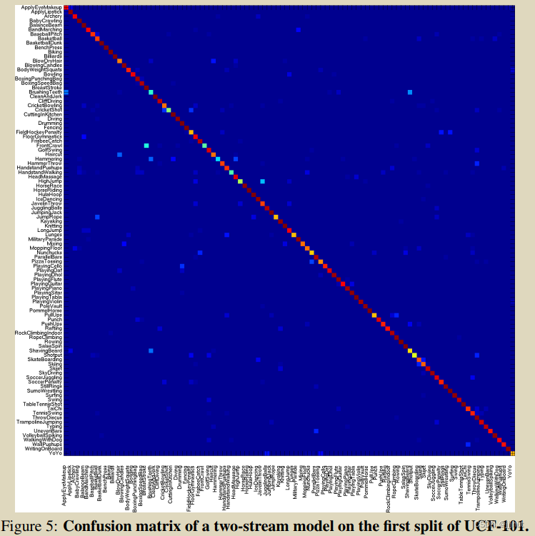
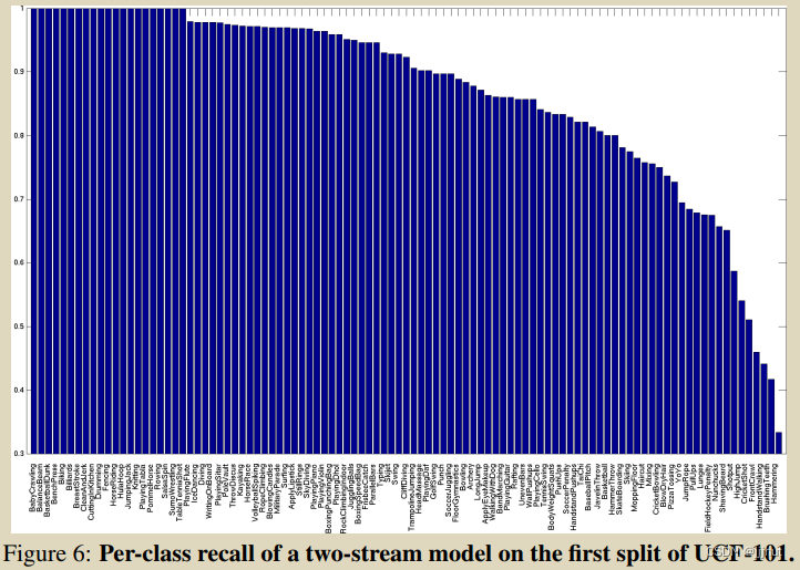
Confusion matrix and per-class recall for UCF-101 classification. In Fig. 5 we show the confusion matrix for UCF-101 classification using our two-stream model, which achieves 87:0% accuracy
on the first dataset split (the last row of Table 3). We also visualise the corresponding per-class recall in Fig. 6.

UCF-101分类的混淆矩阵和每类回忆。在图5中，我们使用我们的双流模型显示了UCF-101分类的混淆矩阵，该模型在第一个数据集分割（表3的最后一行）上实现了87:0%的准确率。我们还在图6中可视化了相应的每类回忆。

The worst class recall corresponds to Hammering class, which is confused with HeadMassage and BrushingTeeth classes. We found that this is due to two reasons. First, the spatial ConvNet confuses Hammering with HeadMassage, which can be caused by the significant presence of human faces in both classes. Second, the temporal ConvNet confuses Hammering with BrushingTeeth, as both actions contain recurring motion patterns (hand moving up and down).

最差的类回忆对应于锤击类，它与头部按摩和刷牙类相混淆。我们发现这有两个原因。首先，空间ConvNet混淆了锤击和头部按摩，这可能是由于两个类别中都存在大量人脸造成的。其次，时态ConvNet混淆了锤击和刷牙，因为这两个动作都包含重复的运动模式（手上下移动）。

7 Conclusions and directions for improvement

We proposed a deep video classification model with competitive performance, which incorporates separate spatial and temporal recognition streams based on ConvNets. Currently it appears that training a temporal ConvNet on optical flow (as here) is significantly better than training on raw stacked frames [14]. The latter is probably too challenging, and might require architectural changes (for example, a combination with the deep matching approach of [30]). Despite using optical flow as input, our temporal model does not require significant hand-crafting, since the flow is computed using a method based on the generic assumptions of constancy and smoothness.

我们提出了一种具有竞争性能的深度视频分类模型，该模型结合了基于ConvNets的独立空间和时间识别流。目前看来，在光流上训练时间ConvNet（如这里所示）明显优于在原始堆叠帧上训练[14]。后者可能太具挑战性，可能需要架构更改（例如，与[30]的深度匹配方法相结合）。尽管使用光流作为输入，但我们的时间模型不需要大量的手工制作，因为流量是使用基于恒定性和平滑性的一般假设的方法计算的。

As we have shown, extra training data is beneficial for our temporal ConvNet, so we are planning to train it on large video datasets, such as the recently released collection of [14]. This, however, poses a significant challenge on its own due to the gigantic amount of training data (multiple TBs).

正如我们所展示的，额外的训练数据对我们的时态ConvNet是有益的，因此我们计划在大型视频数据集上训练它，例如最近发布的[14]的集合。然而，由于大量的训练数据（多个TB），这本身就构成了重大挑战。

There still remain some essential ingredients of the state-of-the-art shallow representation [26], which are missed in our current architecture. The most prominent one is local feature pooling over spatio-temporal tubes, centered at the trajectories. Even though the input (2) captures the optical flow along the trajectories, the spatial pooling in our network does not take the trajectories into account. Another potential area of improvement is explicit handling of camera motion, which in our case is compensated by mean displacement subtraction.

最先进的浅层表示[26]仍然存在一些基本成分，这些成分在我们当前的架构中被遗漏了。最突出的是以轨迹为中心的时空管上的局部特征池。即使输入（2）捕获了沿着轨迹的光流，我们网络中的空间池也没有考虑轨迹。另一个潜在的改进领域是对相机运动的显式处理，在我们的情况下，通过平均位移减法进行补偿。

声明

本文的内容和图来自于论文 Two-Stream Convolutional Networks for Action Recognition in Videos。