推荐阅读列表：

扩散模型实战（一）：基本原理介绍

扩散模型实战（二）：扩散模型的发展

扩散模型实战（三）：扩散模型的应用

扩散模型实战（四）：从零构建扩散模型

扩散模型实战（五）：采样过程

之前的五篇文章主要是为了解释扩散模型的基本概念和流程，使读者更容易理解扩散模型的工作原理，但与实际工作中使用的模型差异较大，从本文开始，我们将初步使用DDPM模型的开源实现库Diffusers，在Diffusers库中DDPM模型的实现库是UNet2DModel

UNet2DModel模型实战

UNet2DModel模型比之前介绍的BasicUNet模型有一些改进，具体如下：

退化过程的处理方式不同，UNet2DModel通过调节时间步来调节噪声量，t作为一个额外参数被传入前向过程；
训练目标不同，UNet2DModel旨在预测不带缩放系数的噪声（也就是单位正太分布的噪声）而不是”去噪“的图像；
UNet2DModel有更多的采样策略可供选择；

下面我们来看一下UNet2DModel的模型参数以及结构，代码如下：

model = UNet2DModel(    sample_size=28,            # 目标图像的分辨率    in_channels=1,         # 输入图像的通道数，RGB图像的通道数为3    out_channels=1,        # 输出图像的通道数    layers_per_block=2,    # 设置要在每一个UNet块中使用多少个ResNet层    block_out_channels=(32, 64, 64), # 与BasicUNet模型的配置基本相同    down_block_types=(         "DownBlock2D",      # 标准的ResNet下采样模块        "AttnDownBlock2D",  # 带有空域维度self-att的ResNet下采样模块        "AttnDownBlock2D",    ),     up_block_types=(        "AttnUpBlock2D",         "AttnUpBlock2D",    # 带有空域维度self-att的ResNet上采样模块        "UpBlock2D",        # 标准的ResNet上采样模块　      ),)　# 输出模型结构（看起来虽然冗长，但非常清晰）print(model)

我们继续来查看一下UNet2DModel模型的参数量，代码如下：

sum([p.numel() for p in model.parameters()]) # UNet2DModel模型使用了大约170万个参数，BasicUNet模型则使用了30多万个参数

# 输出1707009

下面是我们使用UNet2DModel代替BasicUNet模型，重复前面展示的训练以及采样过程（这里t=0，以表明模型是在没有时间步的情况下训练的），完整的代码如下：

#@markdown Trying UNet2DModel instead of BasicUNet:# Dataloader (you can mess with batch size)batch_size = 128train_dataloader = DataLoader(dataset, batch_size=batch_size, shuffle=True)# How many runs through the data should we do?n_epochs = 3# Create the networknet = UNet2DModel(    sample_size=28,  # the target image resolution    in_channels=1,  # the number of input channels, 3 for RGB images    out_channels=1,  # the number of output channels    layers_per_block=2,  # how many ResNet layers to use per UNet block    block_out_channels=(32, 64, 64),  # Roughly matching our basic unet example    down_block_types=(        "DownBlock2D",  # a regular ResNet downsampling block        "AttnDownBlock2D",  # a ResNet downsampling block with spatial self-attention        "AttnDownBlock2D",    ),    up_block_types=(        "AttnUpBlock2D",        "AttnUpBlock2D",  # a ResNet upsampling block with spatial self-attention        "UpBlock2D",   # a regular ResNet upsampling block      ),) #<<<net.to(device)# Our loss finctionloss_fn = nn.MSELoss()# The optimizeropt = torch.optim.Adam(net.parameters(), lr=1e-3)# Keeping a record of the losses for later viewinglosses = []# The training loopfor epoch in range(n_epochs):    for x, y in train_dataloader:        # Get some data and prepare the corrupted version        x = x.to(device) # Data on the GPU        noise_amount = torch.rand(x.shape[0]).to(device) # Pick random noise amounts        noisy_x = corrupt(x, noise_amount) # Create our noisy x        # Get the model prediction        pred = net(noisy_x, 0).sample #<<< Using timestep 0 always, adding .sample        # Calculate the loss        loss = loss_fn(pred, x) # How close is the output to the true 'clean' x?        # Backprop and update the params:        opt.zero_grad()        loss.backward()        opt.step()        # Store the loss for later        losses.append(loss.item())    # Print our the average of the loss values for this epoch:    avg_loss = sum(losses[-len(train_dataloader):])/len(train_dataloader)    print(f'Finished epoch {epoch}. Average loss for this epoch: {avg_loss:05f}')# Plot losses and some samplesfig, axs = plt.subplots(1, 2, figsize=(12, 5))# Lossesaxs[0].plot(losses)axs[0].set_ylim(0, 0.1)axs[0].set_title('Loss over time')# Samplesn_steps = 40x = torch.rand(64, 1, 28, 28).to(device)for i in range(n_steps):  noise_amount = torch.ones((x.shape[0], )).to(device) * (1-(i/n_steps)) # Starting high going low  with torch.no_grad():    pred = net(x, 0).sample  mix_factor = 1/(n_steps - i)  x = x*(1-mix_factor) + pred*mix_factoraxs[1].imshow(torchvision.utils.make_grid(x.detach().cpu(), nrow=8)[0].clip(0, 1), cmap='Greys')axs[1].set_title('Generated Samples');

# 输出Finished epoch 0. Average loss for this epoch: 0.020033Finished epoch 1. Average loss for this epoch: 0.013243Finished epoch 2. Average loss for this epoch: 0.011795

可以看出，比BasicUNet网络生成的结果要好一些。

DDPM原理

论文名称：《Denoising Diffusion Probabilistic Models》

论文地址：https://arxiv.org/pdf/2006.11239.pdf

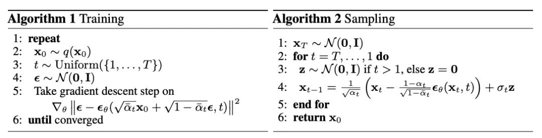
下面是DDPM论文中的公式，Training步骤其实是退化过程，给原始图像逐渐添加噪声的过程，预测目标是拟合每个时间步的采样噪声。

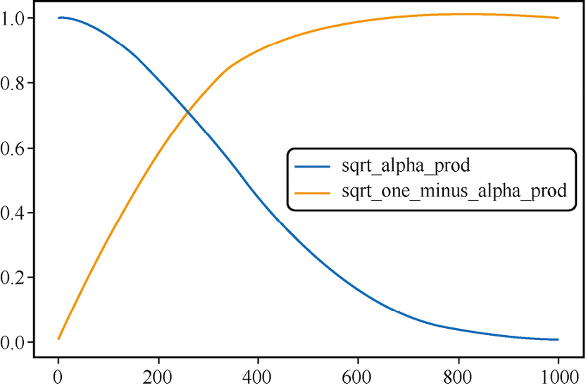
还有一点非常重要：我们都知道在前向过程中是不断添加噪声的，其实这个噪声的系数不是固定的，而是与时间t线性增加的（也成为扩散率），这样的好处是在后向过程开始过程先把"明显"的噪声给去除，对应着较大的扩散率；当去到一定程度，逐渐逼近真实真实图像的时候，去噪速率逐渐减慢，开始微调，也就是对应着较小的扩散率。

下面我们使用代码来看一下输入数据与噪声在不同迭代周期的变化：

noise_scheduler = DDPMScheduler(num_train_timesteps=1000)plt.plot(noise_scheduler.alphas_cumprod.cpu() ** 0.5, label=r"${ \sqrt{\bar{\alpha}_t}}$")plt.plot((1 - noise_scheduler.alphas_cumprod.cpu()) ** 0.5,  label=r"$\sqrt{(1 - \bar{\alpha}_t)}$")plt.legend(fontsize="x-large");

生成的结果，如下图所示：

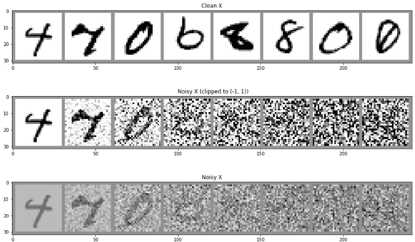
下面我们来看一下，噪声系数不变与DDPM中的噪声方式在MNIST数据集上的加噪效果：

# 可视化：DDPM加噪过程中的不同时间步# 对一批图片加噪，看看效果fig, axs = plt.subplots(3, 1, figsize=(16, 10))xb, yb = next(iter(train_dataloader))xb = xb.to(device)[:8]xb = xb * 2. - 1. # 映射到(-1,1)print('X shape', xb.shape)　# 展示干净的原始输入axs[0].imshow(torchvision.utils.make_grid(xb[:8])[0].detach().    cpu(), cmap='Greys')axs[0].set_title('Clean X')　# 使用调度器加噪timesteps = torch.linspace(0, 999, 8).long().to(device)noise = torch.randn_like(xb) # <<注意是使用randn而不是randnoisy_xb = noise_scheduler.add_noise(xb, noise, timesteps)print('Noisy X shape', noisy_xb.shape)　# 展示“带噪”版本（使用或不使用截断函数clipping）axs[1].imshow(torchvision.utils.make_grid(noisy_xb[:8])[0].detach().cpu().clip(-1, 1), cmap='Greys')axs[1].set_title('Noisy X (clipped to (-1, 1))')axs[2].imshow(torchvision.utils.make_grid(noisy_xb[:8])[0].   detach().cpu(), cmap='Greys')axs[2].set_title('Noisy X');X shape torch.Size([8, 1, 28, 28])Noisy X shape torch.Size([8, 1, 28, 28])