💥💥💞💞欢迎来到本博客❤️❤️💥💥
🏆博主优势:🌞🌞🌞博客内容尽量做到思维缜密,逻辑清晰,为了方便读者。
⛳️座右铭:行百里者,半于九十。
📋📋📋本文目录如下:🎁🎁🎁
目录
💥1 概述
📚2 运行结果
🎉3 参考文献
🌈4 Matlab代码及详细文章
💥1 概述
文献来源:

这项工作提出了一类检测和表征暂态响应测量非线性的时频方法。这些方法适用于响应随着响应幅度的衰减而变得越来越线性的系统。响应数据的离散傅里叶变换是在初始响应的各个部分都为零的情况下得到的。这些频率响应,被称为零早期快速傅立叶变换(ZEFFTs),获得线性频率响应函数(frf)的通常形状,因为更多的初始非线性响应被取消。因此,非线性是由一个质变的形状的ZEFFT作为初始无效部分的长度变化证明。这些光谱显示出对非线性的敏感性,即使它仅在响应的前几个周期中活跃,也能显示出它的存在,就像机械关节的宏观滑移一样。它们还提供了对非线性特性的洞察,潜在地揭示了模态之间的非线性能量传递或系统线性行为的模态振幅。在某些情况下,人们可以从后期线性响应中识别线性模型,并使用它来重建系统在以前的时间执行的响应,如果它是线性的。这表明了非线性的严重程度及其对测量响应的影响。用滑移或冲击非线性系统的分析和实验数据验证了这些方法。
原文摘要:
This work presents a class of time-frequency methods for detecting and characterizing
nonlinearity in transient response measurements. The methods are intended for systems whose response becomes increasingly linear as the response amplitude decays. The discrete Fourier Transform of the response data is found with various sections of the initial response set to zero. These frequency responses, dubbed Zeroed Early-time Fast Fourier Transforms (ZEFFTs), acquire the usual shape of linear Frequency Response Functions (FRFs) as more of the initial nonlinear response is nullified. Hence, nonlinearity is evidenced by a qualitative change in the shape of the ZEFFT as the length of the initial nullified section is varied. These spectra are shown to be sensitive to nonlinearity, revealing its presence even if it is active in only the first few cycles of a response, as may be the case with macro-slip in mechanical joints. They also give insight into the character of the nonlinearity, potentially revealing nonlinear energy transfer between modes or the modal amplitudes below which a system behaves linearly. In some cases one can identify a linear model from the late time, linear response, and use it to reconstruct the response that the system would have executed at previous times if it had been linear.
This gives an indication of the severity of the nonlinearity and its effect on the measured response. The methods are demonstrated on both analytical and experimental data from systems with slip or impact nonlinearities.
📚2 运行结果


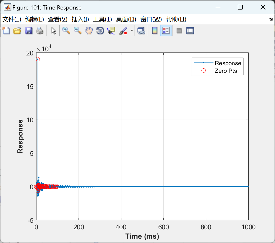


部分代码:
% Specify how systems are connected
at_ns = [2,6]; % attachment happens between this pair of nodes.
fext_ns = 5; % Node at which external force is applied
fnl_vec = zeros(Ntot,1); fnl_vec(at_ns(1)) = -1; fnl_vec(at_ns(2)) = 1;
fext_vec = zeros(Ntot,1); fext_vec(fext_ns(1)) = 1;
dnodes = [1:Ntot];
vnodes = [(Ntot+1):(Ntot*2)];
% Damping Matrix
cfactk = 0.00003; % multiplied by K to get damping.
cfactm = 8; % Multiplied by M to get damping
% for k = 1:5; eval(['c',num2str(k),' = cfact*k',num2str(k),';']); end
C1 = cfactk*K1 + cfactm*M1;
C2 = cfactk*K2 + cfactm*M2; % proportional damping
Ctot = [C1, zeros(size(C1,1),size(C2,2));
zeros(size(C2,1),size(C1,2)), C2];
% Linearized System Analysis %%%%%%%%%%%%%%%%%%%%%%%%%%%%%%%%%%%%%%%%%%
% add a linear spring between attachment nodes
Mlin = Mtot;
Klin = Ktot;
Klin(at_ns,at_ns) = Klin(at_ns,at_ns) + kat*[1, -1; -1, 1];
% Linear Damping matrix:
Clin = Ctot;
Clin(at_ns,at_ns) = Clin(at_ns,at_ns) + cfactk*kat*[1, -1; -1, 1];
% State Space Eigenanalysis
Slin = [Clin, Mlin; Mlin, zeros(size(Mlin))];
Rlin = [-Klin, zeros(size(Mlin));
zeros(size(Mlin)), Mlin];
Alin = (Slin\Rlin);
[Philin,lamlin] = eig(Alin);
lamlin = diag(lamlin);
[junk,sind] = sort(abs(lamlin) - 0.001*min(abs(lamlin))*(imag(lamlin) > 0));
lamlin = lamlin(sind);
Philin = Philin(:,sind);
% % Plot Mode Shapes
% figure(1)
% hls = plot([1:Ntot], imag(Philin(1:Ntot,1:2:end ))); grid on;
% legend(hls, num2str([1:Ntot].'));
% xlabel('X-coordinate');
% ylabel('Im\{Mode Shape\}');
wns = abs(lamlin);
fns = wns/2/pi;
zts = -real(lamlin)./abs(lamlin);
disp('Natural Frequencies:, Damping Ratios:');
[fns, zts]
% DispFnZt(lamlin) - replace 2 lines abouve with this if you have the EMA Functions toolbox
% Nonlinear Parameters
NLType = 'bang'
if strcmp(NLType,'bang');
% Bang (Contact) Nonlinearity
delcont = 1e-3;
k4mult = 20; % Factor by which k4 increases: k4_contact = k4*k4mult
c4mult = 1; % Factor by which c4 increases: c4_contact = c4*c4mult
elseif strcmp(NLType,'cubic');
% Cubic Spring
katnl = 1e8;
else
error('NLType not recognized');
end
% Force paramters
% length of half-sine force pulse
% This is normalized in the EOM to unit area and multiplied by Afnl
tfp = 1e-4;
Afnl = 4e9;
% Which Response to Use in evaluating Nonlinearity (i.e. x1, x2, x3..?)
respind = 6;
% Number of numerical derivatives to evaluate. This M-file simulates
% the displacement response of the 5-DOF system. To simulate the
% measurement of the velocity or acceleration response, the
% displacement response is differentiated using finite differences
% (i.e. Matlab's 'diff' command.) This parameter sets the number of
% derivatives to perform:
nders = 2;
% nders = 0; => use displacement
🎉3 参考文献
部分理论来源于网络,如有侵权请联系删除。


