


核心梯度下降算法:
import numpy as np
from utils.features import prepare_for_training

class LinearRegression:

    def __init__(self,data,labels,polynomial_degree = 0,sinusoid_degree = 0,normalize_data=True):
        """
        1.对数据进行预处理操作
        2.先得到所有的特征个数
        3.初始化参数矩阵
        """
        (data_processed, #预处理完之后的数据(标准化之后的数据)
         features_mean,  #预处理完之后的平均值和标准差
         features_deviation)  = prepare_for_training(data, polynomial_degree, sinusoid_degree,normalize_data=True)
        # 在数据预处理中,对数据进行标准化(normalize)时,通常会使用数据的均值和标准差。标准化是一种常见的数据预处理技术,
        # 它通过减去均值并除以标准差,将数据转换为具有零均值和单位方差的形式。这样做可以使得不同尺度的特征具有相似的重要性,有助于提高模型的性能和收敛速度。

        self.data = data_processed
        self.labels = labels
        self.features_mean = features_mean
        self.features_deviation = features_deviation
        self.polynomial_degree = polynomial_degree
        self.sinusoid_degree = sinusoid_degree
        self.normalize_data = normalize_data

        #所有特征个数
        num_features = self.data.shape[1]

        #最终求解的 theta 值,初始化theta参数矩阵
        self.theta = np.zeros((num_features,1))


    #alpha为学习率,也就是步长,越小越好;num_iterations为迭代次数
    def train(self,alpha,num_iterations = 500):
        """
                    训练模块,执行梯度下降
        """
        #cost_history记录损失变化
        cost_history = self.gradient_descent(alpha,num_iterations)
        return self.theta,cost_history

    #梯度下降
    def gradient_descent(self,alpha,num_iterations):
        """
                    实际迭代模块,会迭代num_iterations次
        """
        #cost_history记录损失变化
        cost_history = []
        for _ in range(num_iterations):
            self.gradient_step(alpha)
            cost_history.append(self.cost_function(self.data,self.labels))
        return cost_history

    #实际参数更新的时候 计算步骤,公式在这里进行计算,梯度下降的核心计算过程
    def gradient_step(self,alpha):
        """
                    梯度下降参数更新计算方法,注意是矩阵运算
        """
        #样本个数
        num_examples = self.data.shape[0]
        #预测值
        prediction = LinearRegression.hypothesis(self.data, self.theta)
        #误差值delta = 预测值-真实值
        delta = prediction - self.labels

        #通过步长来,对theta参数进行迭代更新
        theta = self.theta
        #使用矩阵可以避免for循环
        theta = theta - alpha*(1/num_examples)*(np.dot(delta.T,self.data)).T
        self.theta = theta


    #损失函数计算方法
    def cost_function(self,data,labels):
        """
                    损失计算方法
        """
        num_examples = data.shape[0]
        delta = LinearRegression.hypothesis(self.data,self.theta) - labels
        cost = (1/2)*np.dot(delta.T,delta)/num_examples
        return cost[0][0]


    #预测值 = theta * 数据, 返回矩阵点乘数据    y = theta1*x1 + theta2*x2 + ……
    @staticmethod
    def hypothesis(data,theta):
        predictions = np.dot(data,theta)
        return predictions


    #获取损失值
    def get_cost(self,data,labels):
        data_processed = prepare_for_training(data,
         self.polynomial_degree,
         self.sinusoid_degree,
         self.normalize_data
         )[0]
        return self.cost_function(data_processed,labels)

    #获取预测值
    def predict(self,data):
        """
                    用训练的参数模型,与预测得到回归值结果
        """
        data_processed = prepare_for_training(data,
         self.polynomial_degree,
         self.sinusoid_degree,
         self.normalize_data
         )[0]
        predictions = LinearRegression.hypothesis(data_processed,self.theta)
        return predictions
"""Prepares the dataset for training"""

import numpy as np
from .normalize import normalize
from .generate_sinusoids import generate_sinusoids
from .generate_polynomials import generate_polynomials


def prepare_for_training(data, polynomial_degree=0, sinusoid_degree=0, normalize_data=True):

    # 计算样本总数
    num_examples = data.shape[0]

    data_processed = np.copy(data)

    # 预处理
    features_mean = 0
    features_deviation = 0
    data_normalized = data_processed
    if normalize_data:
        (
            data_normalized,
            features_mean,
            features_deviation
        ) = normalize(data_processed)

        data_processed = data_normalized

    # 特征变换sinusoidal
    if sinusoid_degree > 0:
        sinusoids = generate_sinusoids(data_normalized, sinusoid_degree)
        data_processed = np.concatenate((data_processed, sinusoids), axis=1)

    # 特征变换polynomial
    if polynomial_degree > 0:
        polynomials = generate_polynomials(data_normalized, polynomial_degree, normalize_data)
        data_processed = np.concatenate((data_processed, polynomials), axis=1)

    # 加一列1
    data_processed = np.hstack((np.ones((num_examples, 1)), data_processed))

    return data_processed, features_mean, features_deviation
绘图:
import numpy as np
import pandas as pd
import matplotlib.pyplot as plt

from linear_regression import LinearRegression

data = pd.read_csv('../data/world-happiness-report-2017.csv')

# 得到训练和测试数据
train_data = data.sample(frac = 0.8)
test_data = data.drop(train_data.index)

input_param_name = 'Economy..GDP.per.Capita.'
output_param_name = 'Happiness.Score'

x_train = train_data[[input_param_name]].values
y_train = train_data[[output_param_name]].values

x_test = test_data[input_param_name].values
y_test = test_data[output_param_name].values

plt.scatter(x_train,y_train,label='Train data')
plt.scatter(x_test,y_test,label='test data')
plt.xlabel(input_param_name)
plt.ylabel(output_param_name)
plt.title('Happy')
plt.legend()
plt.show()

num_iterations = 500
learning_rate = 0.01

linear_regression = LinearRegression(x_train,y_train)
(theta,cost_history) = linear_regression.train(learning_rate,num_iterations)

print ('开始时的损失:',cost_history[0])
print ('训练后的损失:',cost_history[-1])

plt.plot(range(num_iterations),cost_history)
plt.xlabel('Iter')
plt.ylabel('cost')
plt.title('GD')
plt.show()

predictions_num = 100
x_predictions = np.linspace(x_train.min(),x_train.max(),predictions_num).reshape(predictions_num,1)
y_predictions = linear_regression.predict(x_predictions)

plt.scatter(x_train,y_train,label='Train data')
plt.scatter(x_test,y_test,label='test data')
plt.plot(x_predictions,y_predictions,'r',label = 'Prediction')
plt.xlabel(input_param_name)
plt.ylabel(output_param_name)
plt.title('Happy')
plt.legend()
plt.show() 

两个变量的线性回归模型,建议使用plotly进行绘图
import numpy as np
import pandas as pd
import matplotlib.pyplot as plt
import plotly
import plotly.graph_objs as go

plotly.offline.init_notebook_mode()
from linear_regression import LinearRegression

data = pd.read_csv('../data/world-happiness-report-2017.csv')

train_data = data.sample(frac=0.8)
test_data = data.drop(train_data.index)

input_param_name_1 = 'Economy..GDP.per.Capita.'
input_param_name_2 = 'Freedom'
output_param_name = 'Happiness.Score'


x_train = train_data[[input_param_name_1, input_param_name_2]].values
y_train = train_data[[output_param_name]].values

x_test = test_data[[input_param_name_1, input_param_name_2]].values
y_test = test_data[[output_param_name]].values

# Configure the plot with training dataset.
plot_training_trace = go.Scatter3d(
    x=x_train[:, 0].flatten(),
    y=x_train[:, 1].flatten(),
    z=y_train.flatten(),
    name='Training Set',
    mode='markers',
    marker={
        'size': 10,
        'opacity': 1,
        'line': {
            'color': 'rgb(255, 255, 255)',
            'width': 1
        },
    }
)


plot_test_trace = go.Scatter3d(
    x=x_test[:, 0].flatten(),
    y=x_test[:, 1].flatten(),
    z=y_test.flatten(),
    name='Test Set',
    mode='markers',
    marker={
        'size': 10,
        'opacity': 1,
        'line': {
            'color': 'rgb(255, 255, 255)',
            'width': 1
        },
    }
)


plot_layout = go.Layout(
    title='Date Sets',
    scene={
        'xaxis': {'title': input_param_name_1},
        'yaxis': {'title': input_param_name_2},
        'zaxis': {'title': output_param_name}
    },
    margin={'l': 0, 'r': 0, 'b': 0, 't': 0}
)

plot_data = [plot_training_trace, plot_test_trace]

plot_figure = go.Figure(data=plot_data, layout=plot_layout)

plotly.offline.plot(plot_figure)

num_iterations = 500
learning_rate = 0.01
polynomial_degree = 0
sinusoid_degree = 0

linear_regression = LinearRegression(x_train, y_train, polynomial_degree, sinusoid_degree)

(theta, cost_history) = linear_regression.train(
    learning_rate,
    num_iterations
)

print('开始损失',cost_history[0])
print('结束损失',cost_history[-1])

plt.plot(range(num_iterations), cost_history)
plt.xlabel('Iterations')
plt.ylabel('Cost')
plt.title('Gradient Descent Progress')
plt.show()

predictions_num = 10

x_min = x_train[:, 0].min();
x_max = x_train[:, 0].max();

y_min = x_train[:, 1].min();
y_max = x_train[:, 1].max();


x_axis = np.linspace(x_min, x_max, predictions_num)
y_axis = np.linspace(y_min, y_max, predictions_num)


x_predictions = np.zeros((predictions_num * predictions_num, 1))
y_predictions = np.zeros((predictions_num * predictions_num, 1))

x_y_index = 0
for x_index, x_value in enumerate(x_axis):
    for y_index, y_value in enumerate(y_axis):
        x_predictions[x_y_index] = x_value
        y_predictions[x_y_index] = y_value
        x_y_index += 1

z_predictions = linear_regression.predict(np.hstack((x_predictions, y_predictions)))

plot_predictions_trace = go.Scatter3d(
    x=x_predictions.flatten(),
    y=y_predictions.flatten(),
    z=z_predictions.flatten(),
    name='Prediction Plane',
    mode='markers',
    marker={
        'size': 1,
    },
    opacity=0.8,
    surfaceaxis=2,
)

plot_data = [plot_training_trace, plot_test_trace, plot_predictions_trace]
plot_figure = go.Figure(data=plot_data, layout=plot_layout)
plotly.offline.plot(plot_figure) 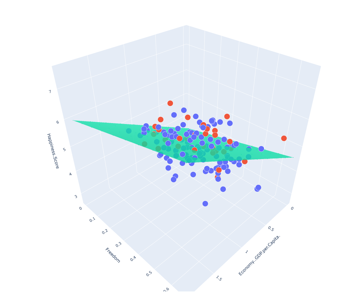


![[PCIE体系结构导读]PCIE总结(一)](https://img-blog.csdnimg.cn/ba8ef07dc650433cbe73288e8f0658b2.png)