【无线传感器】使用 MATLAB和 XBee连续监控温度传感器无线网络研究（Matlab代码实现）

💥💥💞💞欢迎来到本博客❤️❤️💥💥

🏆博主优势：🌞🌞🌞博客内容尽量做到思维缜密，逻辑清晰，为了方便读者。

⛳️座右铭：行百里者，半于九十。

📋📋📋本文目录如下：🎁🎁🎁

目录

💥1 概述

📚2 运行结果

🎉3 参考文献

🌈4 Matlab代码及数据

💥1 概述

在本文中，MATLAB 用于通过与使用 XBee 系列 2 模块构建的温度传感器无线网络进行交互，连续监控整个公寓的温度。每个XBee边缘节点从多个温度传感器读取模拟电压（与温度成线性比例）。读数通过协调器XBee模块传输回MATLAB。本文说明了如何操作、获取和分析来自连接到多个 XBee 边缘节点的多个传感器网络的数据。数据采集时间从数小时到数天不等，以帮助设计和构建智能恒温器系统。

📚2 运行结果

部分代码：

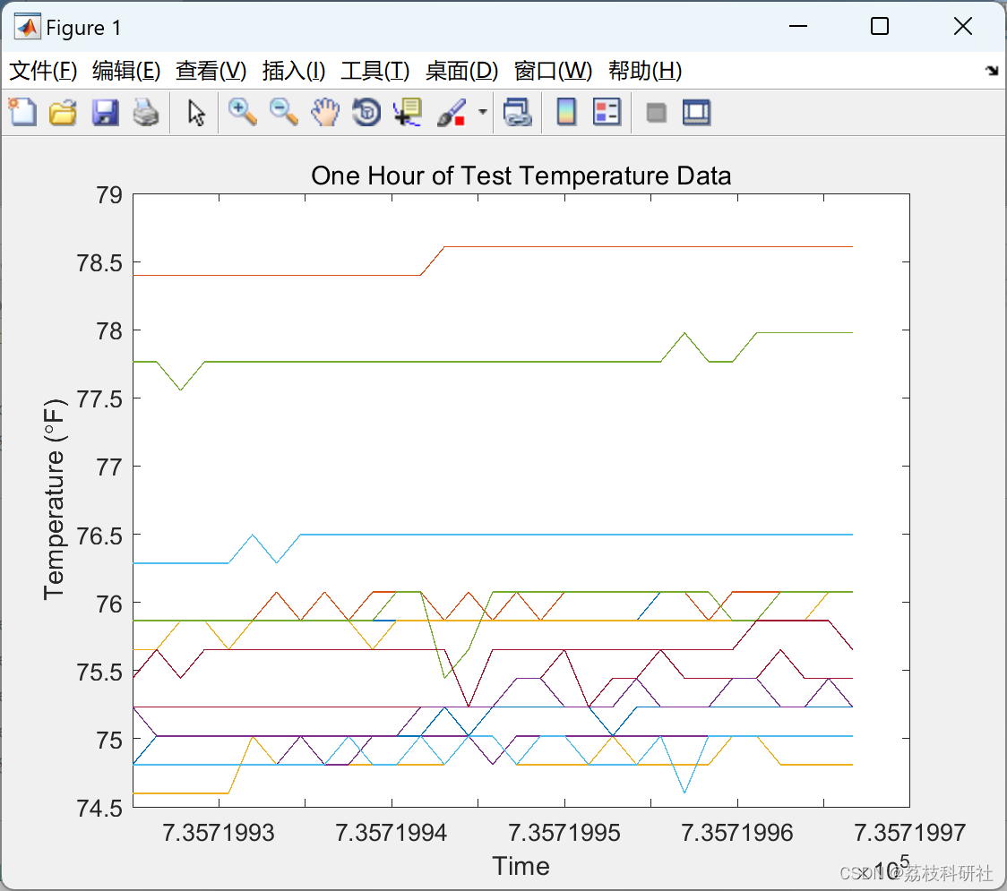
%% Overview of Data
% As I mentioned in a previous post, I collected the temperature every two
% minutes over the course of 9 days. I placed 14 sensors in my apartment: 9
% located inside, 2 located outside, and 3 located in radiators. The data
% is stored in the file <../twoweekstemplog.txt |twoweekstemplog.txt|>.

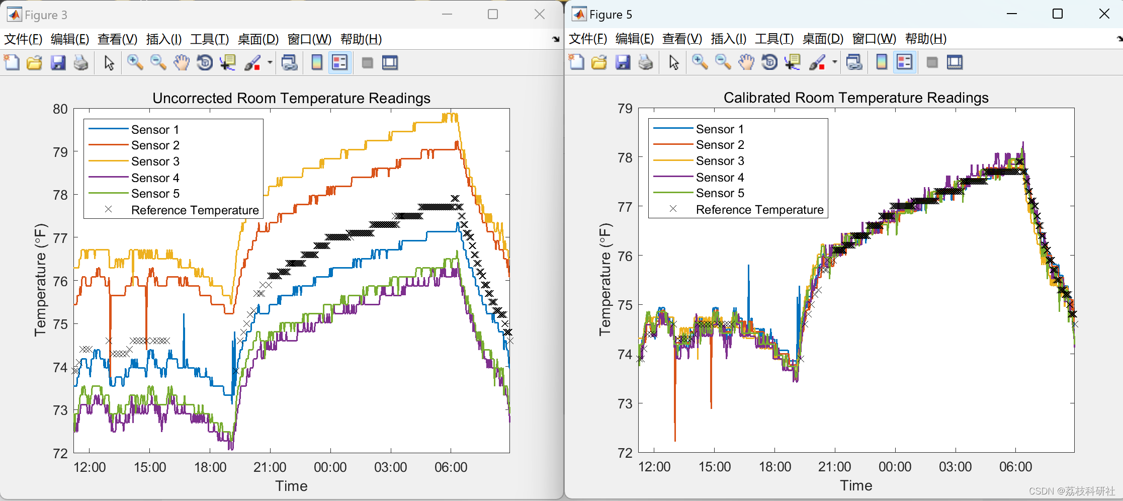
[tempF,ts,location,lineSpecs] = XBeeReadLog('twoweekstemplog.txt',60);
tempF = calibrateTemperatures(tempF);
plotTemps(ts,tempF,location,lineSpecs)
legend('off')
xlabel('Date')
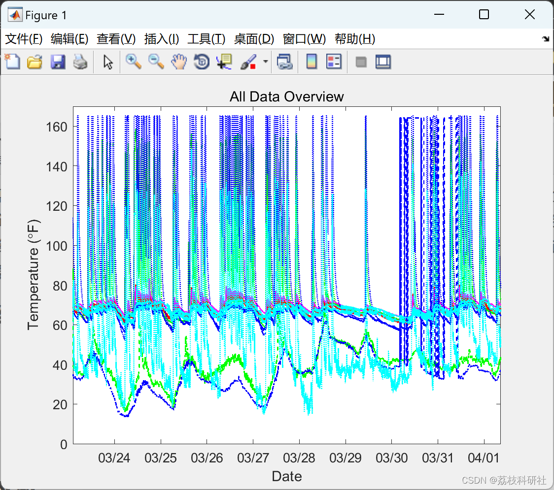
title('All Data Overview')

%%
% _Figure 1: All temperature data from a 9 day period._
%
% That graph is a bit too cluttered to be very meaningful. Let me remove
% the radiator data and the legend and see if that helps.

notradiator = [1 2 3 5 6 7 8 9 10 12 13];
plotTemps(ts,tempF(:,notradiator),location(notradiator),lineSpecs(notradiator,:))
legend('off')
xlabel('Date')
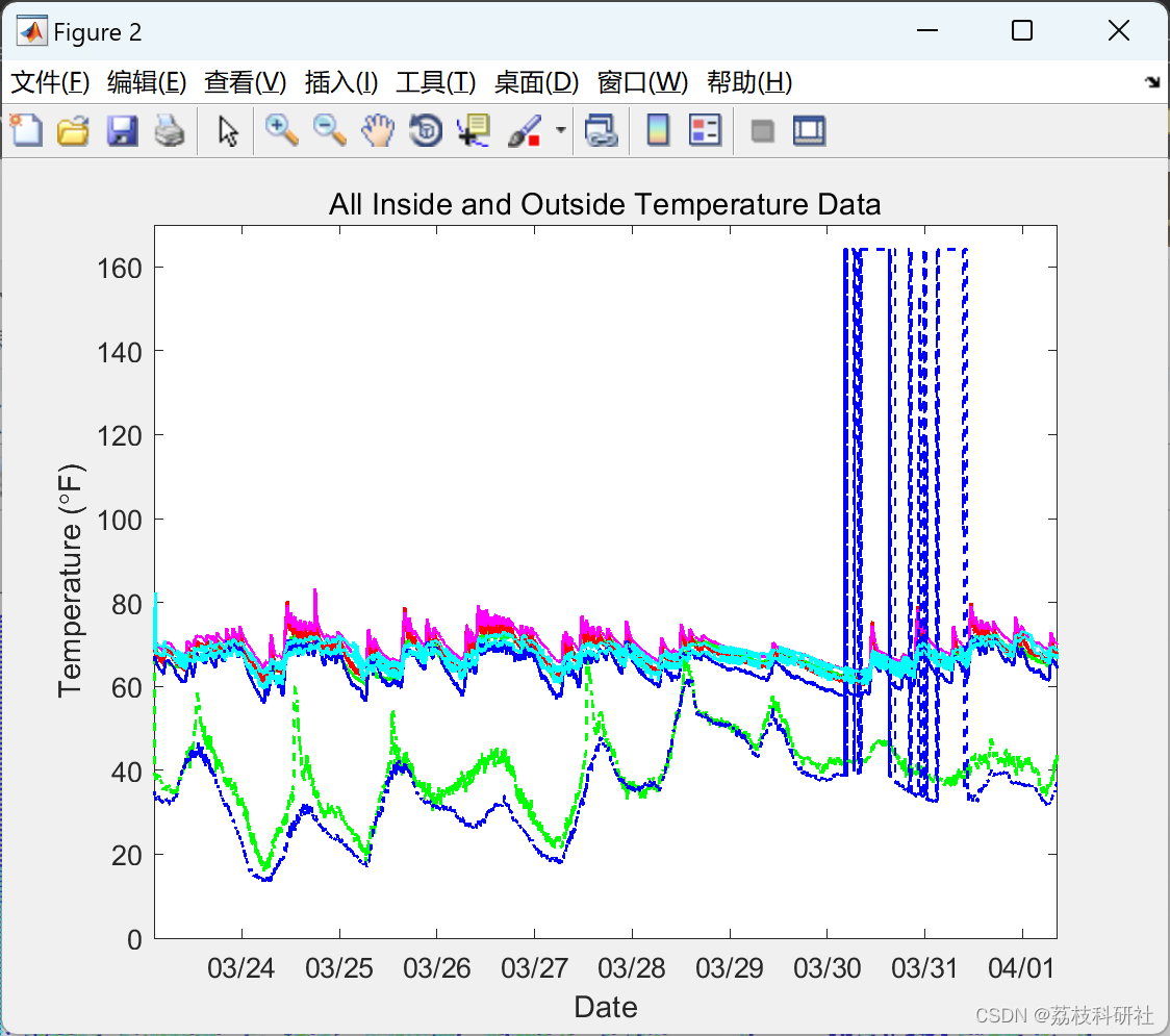
title('All Inside and Outside Temperature Data')

%%
% _Figure 2: Just inside and outside temperature data, with radiator data removed._
%
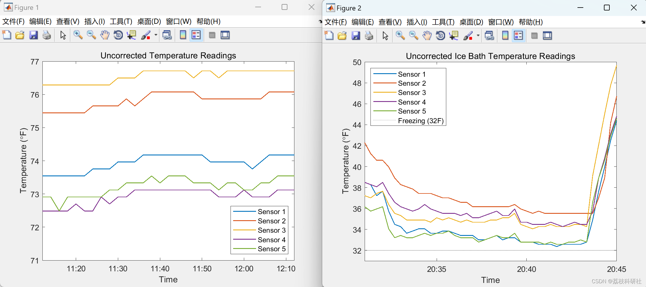
% Now I can see some places where one of the outdoor temperature sensors
% (blue line) gave erroneous data, so let's remove those data points. This
% data was collected in March in Massachusetts, so I can safely assume the
% outdoor temperature never reached 80 F. I replaced any values above 80 F
% with |NaN| (not-a-number) so they are ignored in further analysis.

outside = [3 10];
outsideTemps = tempF(:,outside);
toohot = outsideTemps>80;
outsideTemps(toohot) = NaN;
tempF(:,outside) = outsideTemps;

plotTemps(ts,tempF(:,notradiator),location(notradiator),lineSpecs(notradiator,:))
legend('off')
xlabel('Date')
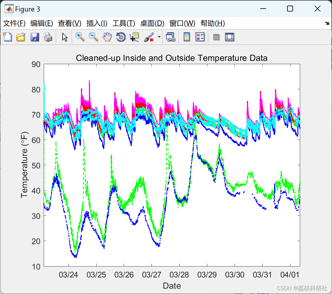
title('Cleaned-up Inside and Outside Temperature Data')

%%
% _Figure 3: Inside and outside temperature data with erroneous data removed._
%
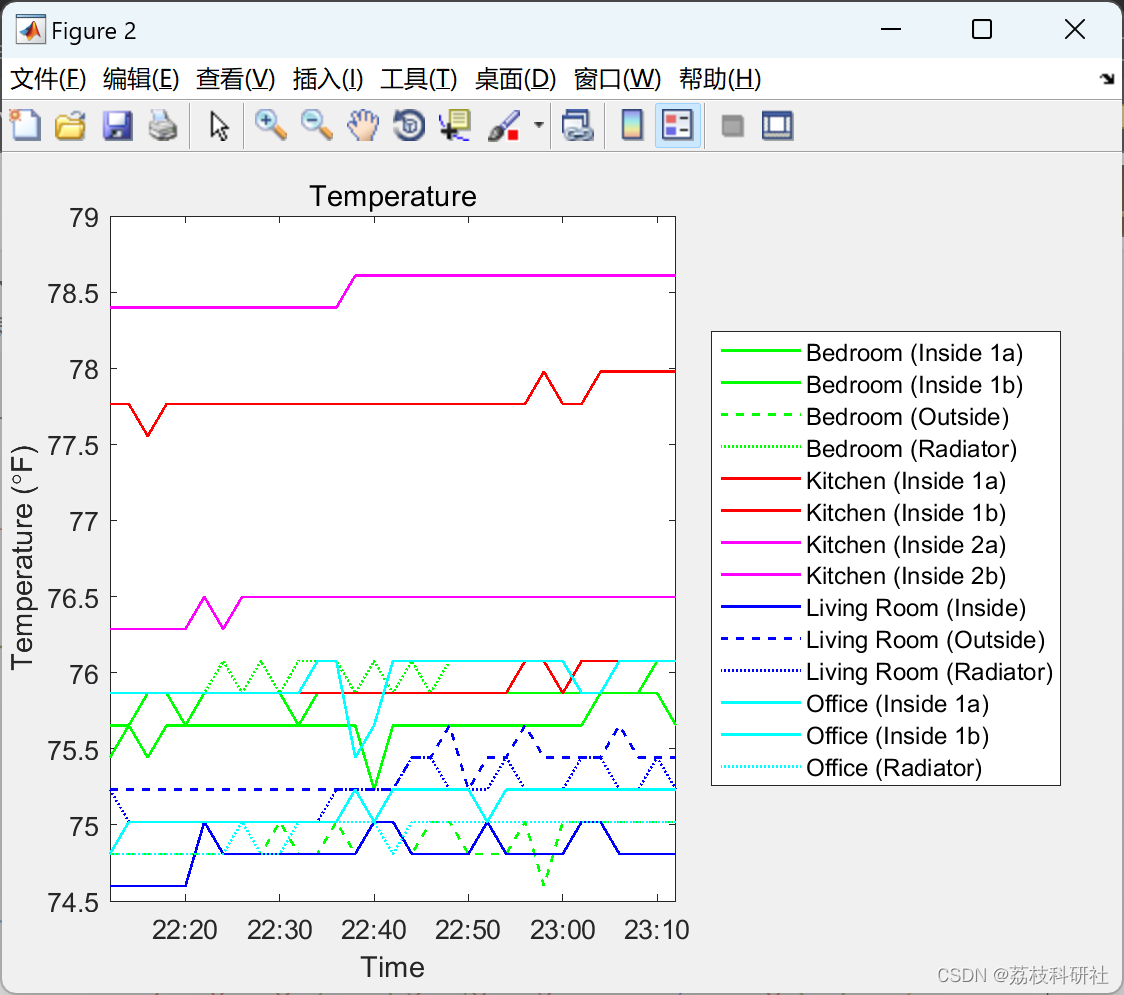
% I'll also remove all but one inside sensor per room, and give the
% remaining sensors shorter names, to keep the graph from getting too
% cluttered.

show = [1 5 9 12 10 3];
location(show) = ...
{'Bedroom','Kitchen','Living Room','Office','Front Porch','Side Yard'}';

plotTemps(ts,tempF(:,show),location(show),lineSpecs(show,:))
ylim([0 90])
legend('Location','SouthEast')
xlabel('Date')
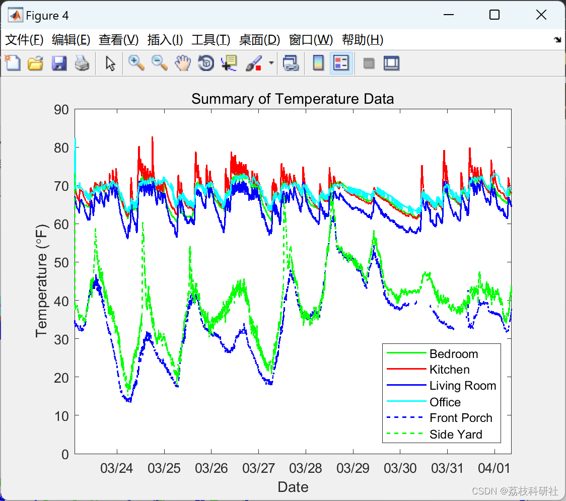
title('Summary of Temperature Data')

%%
% _Figure 4: Summary of temperature data with only one inside temperature
% sensor per room with outside temperatures._
%
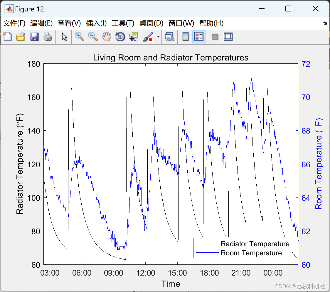
% That looks much better. This data was collected over the course of 9
% days, and the first thing that stands out to me is the periodic outdoor
% temperature, which peaks every day at around noon. I also notice a sharp
% spike in the side yard (green) temperature on most days. My front porch
% (blue) is located on the north side of my apartment, and does not get
% much sun. My side yard is on the east side of my apartment, and that
% spike probably corresponds to when the sun hits the sensor from between
% my apartment and the building next door.

%% When do my radiators start to heat up?
% The radiator temperature can be used to measure how long it takes for my
% boiler and radiators to warm up after the heat has been turned on. Let's
% take a look at 1 day of data from the living room radiator:

% Grab the Living Room Radiator Temperature (index 11) from the |tempF| matrix.
radiatorTemp = tempF(:,11);

% Fill in any missing values:
validts = ts(~isnan(radiatorTemp));
validtemp = radiatorTemp(~isnan(radiatorTemp));
nants = ts(isnan(radiatorTemp));
radiatorTemp(isnan(radiatorTemp)) = interp1(validts,validtemp,nants);

% Plot the data
oneday = [ts(1) ts(1)+1];
figure
plot(ts,radiatorTemp,'k.-')
xlim(oneday)
xlabel('Time')
ylabel('Radiator Temperature (\circF)')
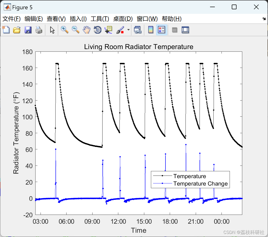
title('Living Room Radiator Temperature')
datetick('keeplimits')
snapnow

%%
% _Figure 5: One day of temperature data from the living room radiator._
%
% As expected, I see a sharp rise in the radiator temperature, followed by
% a short leveling off (when the radiator temperature maxes out the
% temperature sensor), and finally a gradual cooling of the radiator. Let
% me superimpose the rate of change in temperature onto the plot.

tempChange = diff([NaN; radiatorTemp]);

hold on
plot(ts,tempChange,'b.-')
legend({'Temperature', 'Temperature Change'},'Location','Best')

%%
% _Figure 6: One day of data from the living room radiator with temperature change._
%
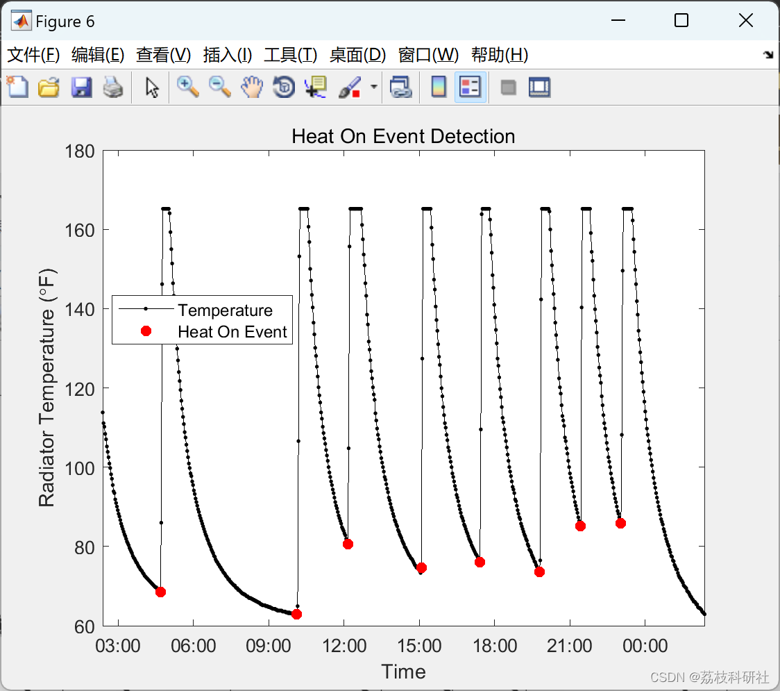
% It looks like I can detect those peaks by looking for large jumps in the
% temperature. After some trial and error, I settled on three criteria to
% identify when the heat comes on:
%
% # Change in temperature greater than four times the previous change in temperature.
% # Change in temperature of more than 1 degree F.
% # Keep the first in a sequence of matching points (remove doubles)

fourtimes = [tempChange(2:end)>abs(4*tempChange(1:end-1)); false];
greaterthanone = [tempChange(2:end)>1; false];
heaton = fourtimes & greaterthanone;
doubles = [false; heaton(2:end) & heaton(1:end-1)];
heaton(doubles) = false;

%%
% Let's see how well I detected those peaks by superimposing red dots over
% the times I detected.

figure
plot(ts,radiatorTemp,'k.-')
hold on
plot(ts(heaton),radiatorTemp(heaton),'r.','MarkerSize',20)
xlim(oneday);
datetick('keeplimits')
xlabel('Time')
ylabel('Radiator Temperature (\circF)')
title('Heat On Event Detection')
legend({'Temperature', 'Heat On Event'},'Location','Best')

%%
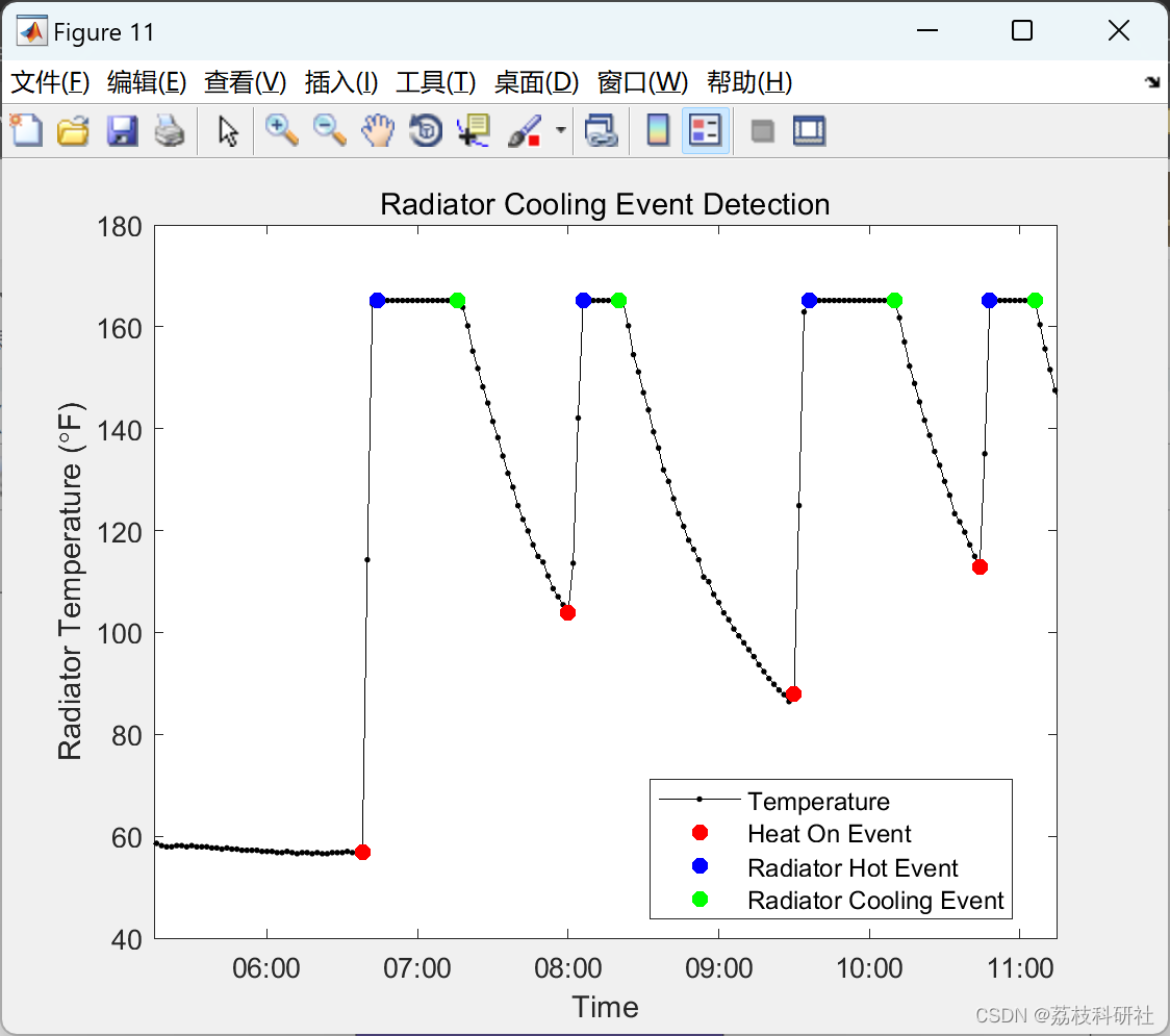
% _Figure 7: Radiator temperature with heating events marked with red dots._
%
% Looks pretty good, which means now I have a list of all the times that
% the heat came on in my apartment.
heatontimes = ts(heaton);

%% How long does it take for my heat to turn on?
% I currently have a programmable 5/2 thermostat, which means I can set
% one program for weekdays (Monday through Friday) and one program for both
% Saturday and Sunday. I know my thermostat is set to go down to 62 at
% night, and back up to 68 at 6:15am Monday through Friday and 10:00am on
% Saturday and Sunday. I used that knowledge to determine how long after my
% thermostat activates that my radiators warm up.
%
% I started by creating a vector of all the days in the test period. I
% removed Monday because I manually turned on the thermostat early that day.
mornings = floor(min(ts)):floor(max(ts));
mornings(2) = []; % Remove Monday

%%
% Then I added either 6:15am or 10:00am to each day depending on whether it
% was a weekday or a weekend.
isweekend = weekday(mornings) == 1 | weekday(mornings) == 7;
mornings(isweekend) = mornings(isweekend)+10/24; % 10:00 AM
mornings(~isweekend) = mornings(~isweekend)+6.25/24; % 6:15 AM

%%
% Next I looked for the first time the heat came on after the programmed
% time each morning.
heatontimes_mat = repmat(heatontimes,1,length(mornings));
mornings_mat = repmat(mornings,length(heatontimes),1);
timelag = heatontimes_mat - mornings_mat;
timelag(timelag<=0) = NaN;

plot(ts,radiatorTemp,'k.-')
hold on
plot(heatontimes,heatontemp,'r.','MarkerSize',20)
plot(heatontimes(heatind),heatontemp(heatind),'bo','MarkerSize',10)
plot([mornings;mornings],repmat(ylim',1,length(mornings)),'b-');
xlim(onemorning);
datetick('keeplimits')
xlabel('Time')
ylabel('Radiator Temperature (\circF)')
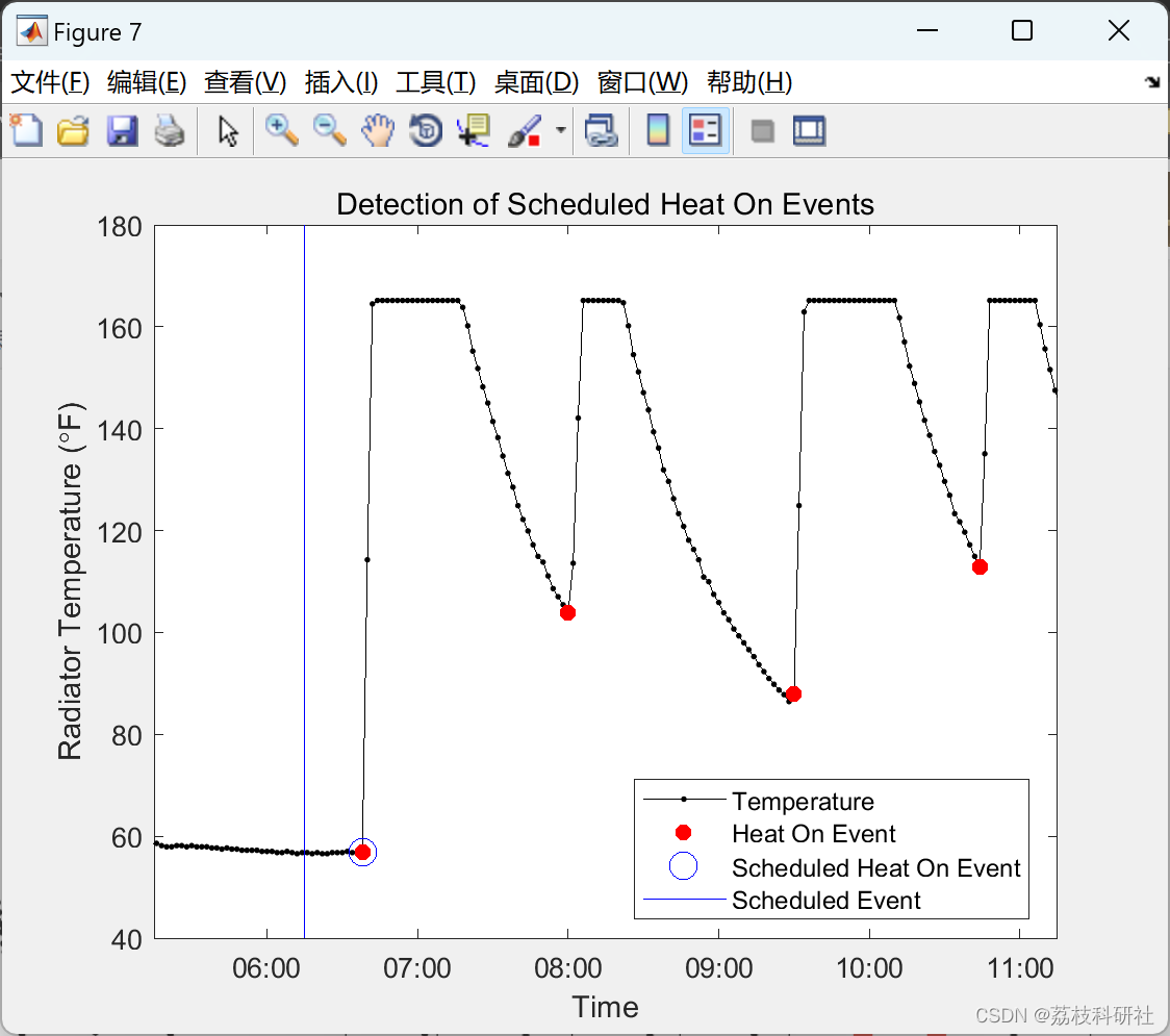
title('Detection of Scheduled Heat On Events')
legend({'Temperature', 'Heat On Event', 'Scheduled Heat On Event',...
'Scheduled Event'},'Location','Best')

%%
% _Figure 8: Six hours of radiator data, with a blue line indicating when
% the thermostat turned on in the morning, and blue circle indicating the
% corresponding heat on event of the radiator._
%
% Let's look at a histogram of those delays:
figure
hist(delay,min(delay):max(delay))
xlabel('Minutes')
ylabel('Frequency')
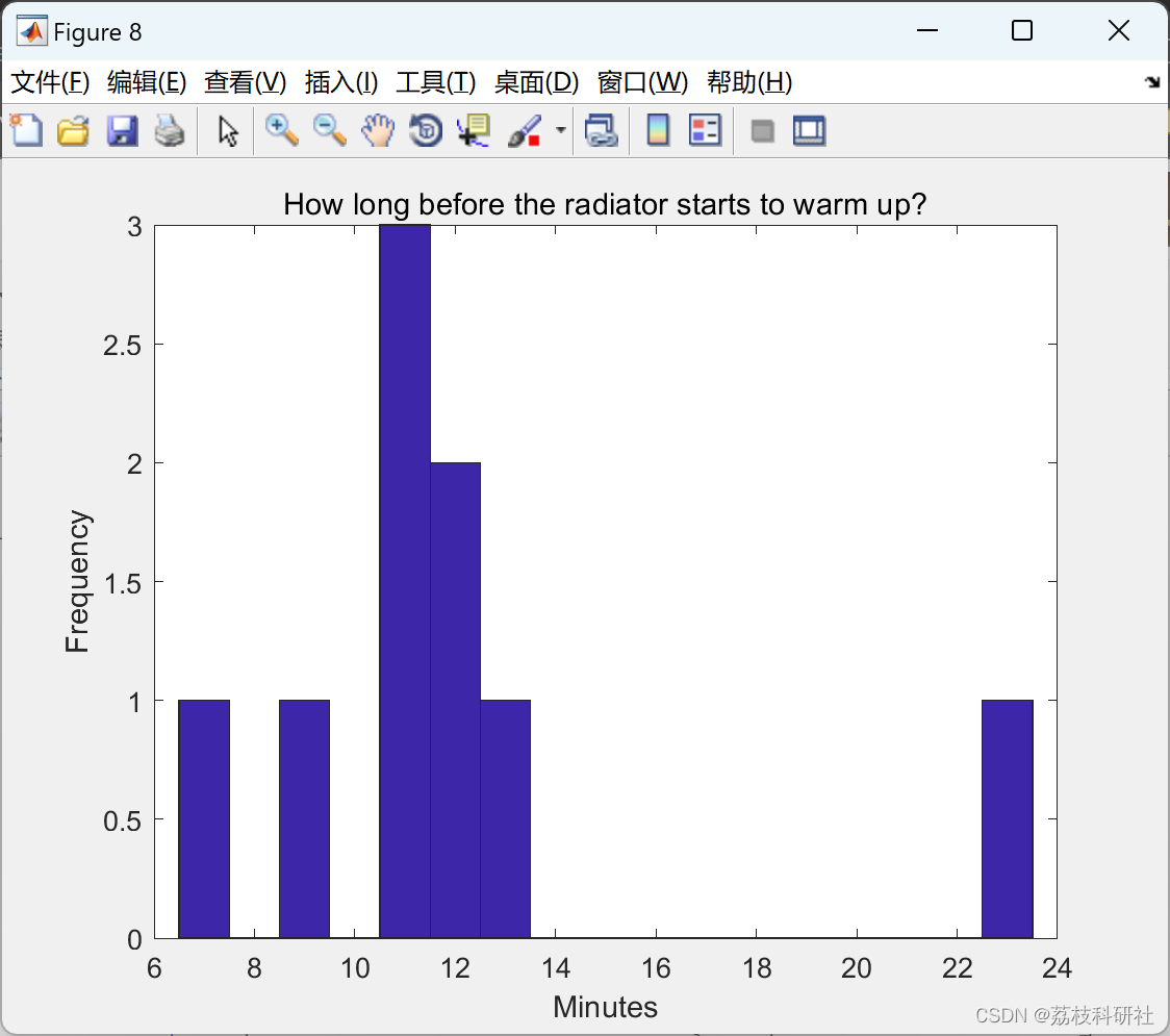
title('How long before the radiator starts to warm up?')

%%
% _Figure 9: Histogram showing delay between thermostat activation and the
% radiators starting to warm up._
%
% It looks like the delay between the thermostat coming on in the morning
% and the radiators starting to warming up can range from 7 minutes to as
% high as 24 minutes, but on average this delay is around 12-13 minutes.
heatondelay = 12;

%% How long does it take for the radiators to warm up?
% Once the radiators start to warm up, it takes a few minutes for them to
% reach full temperature. Let's look at how long this takes. I'll look for
% times when the radiator temperature first maxes out the temperature
% sensor after having been below the maximum for at least 10 minutes (5
% samples).

maxtemp = max(radiatorTemp);
radiatorhot = radiatorTemp(6:end)==maxtemp & ...
radiatorTemp(1:end-5)<maxtemp &...
radiatorTemp(2:end-4)<maxtemp &...
radiatorTemp(3:end-3)<maxtemp &...
radiatorTemp(4:end-2)<maxtemp &...
radiatorTemp(5:end-1)<maxtemp;
radiatorhot = [false(5,1); radiatorhot];
radiatorhottimes = ts(radiatorhot);
%
% Now I'll match the |radiatorhottimes| to the |heatontimes| using the same
% technique I used above.
radiatorhottimes_mat = repmat(radiatorhottimes',length(heatontimes),1);
heatontimes_mat = repmat(heatontimes,1,length(radiatorhottimes));
timelag = radiatorhottimes_mat - heatontimes_mat;
timelag(timelag<=0) = NaN;
[delay, foundmatch] = min(timelag);
delay = round(delay*24*60);

%%
% Let's look at a histogram of those delays:
figure
hist(delay,min(delay):2:max(delay))
xlabel('Minutes');
ylabel('Frequency')
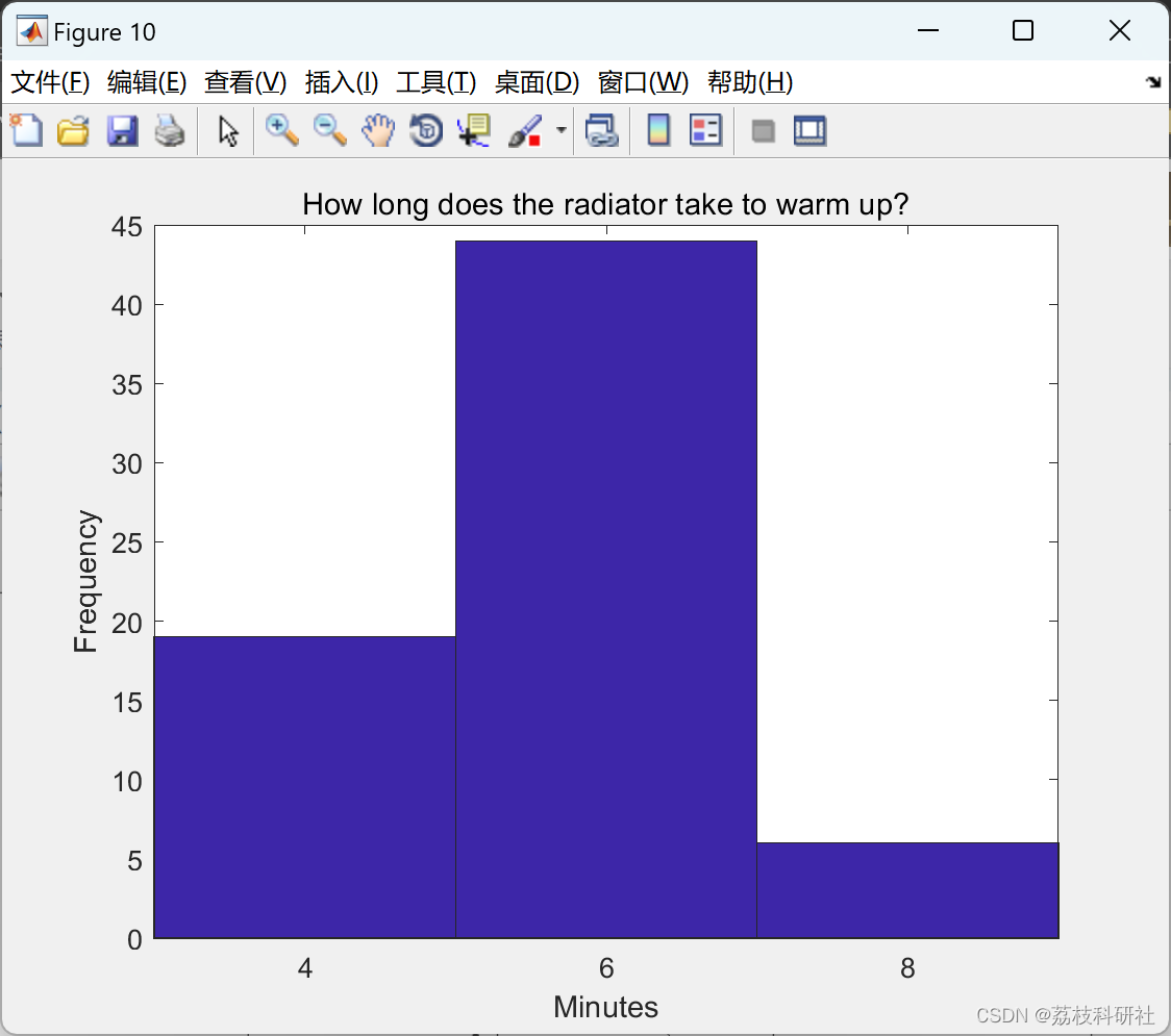
title('How long does the radiator take to warm up?')

%%
% _Figure 11: Histogram showing time required for the radiators to warm up._
%
% It looks like the radiators take between 4 and 8 minutes from when they
% start to warm up until they are at full temperature.
radiatorheatdelay = 6;

%%
% Later on in my analysis, I will only want to use times that the heat came
%
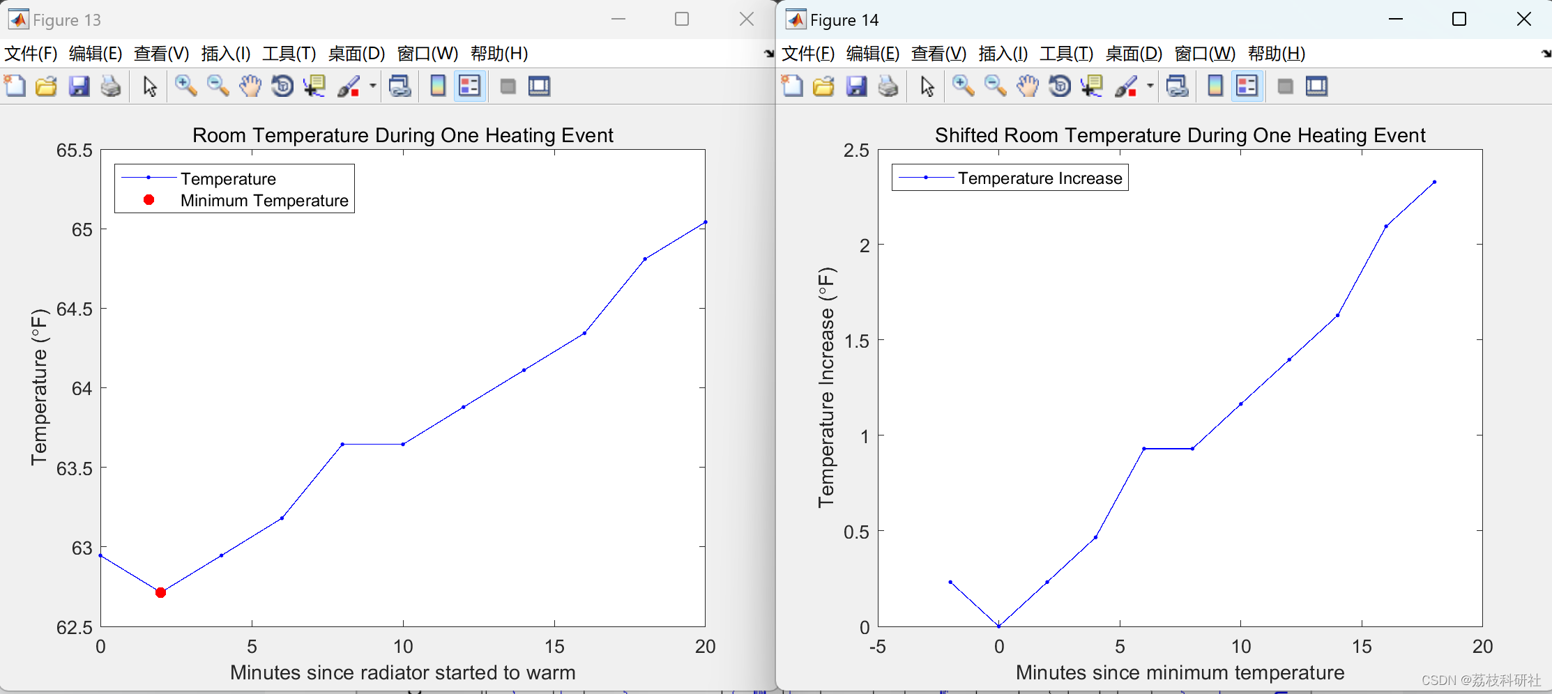
% Although it isn't perfect, it looks close to a linear relationship. Since
% I am interested in the time it takes to reach the desired temperature
% (what could be considered the "specific heat capacity" of the room), let
% me replot the data with time on the y-axis and temperature on the x-axis
% (swapping the axes from the previous figure). I'll also plot the data as
% individual points instead of lines, because that is how the data is going
% to be fed into |polyfit| later.

% Remove temperatures occuring before the minimum temperature.
segmentTempsShifted(segmentTimesShifted<0) = NaN;

figure
h1 = plot(segmentTempsShifted',segmentTimesShifted','k.');
xlabel('Temperature Increase (\circF)')
ylabel('Minutes since minimum temperature')
title('Time to Heat Living Room')
snapnow

%%
% _Figure 17: The time it takes to heat the living room (axes flipped from
% Figure 16)._
%
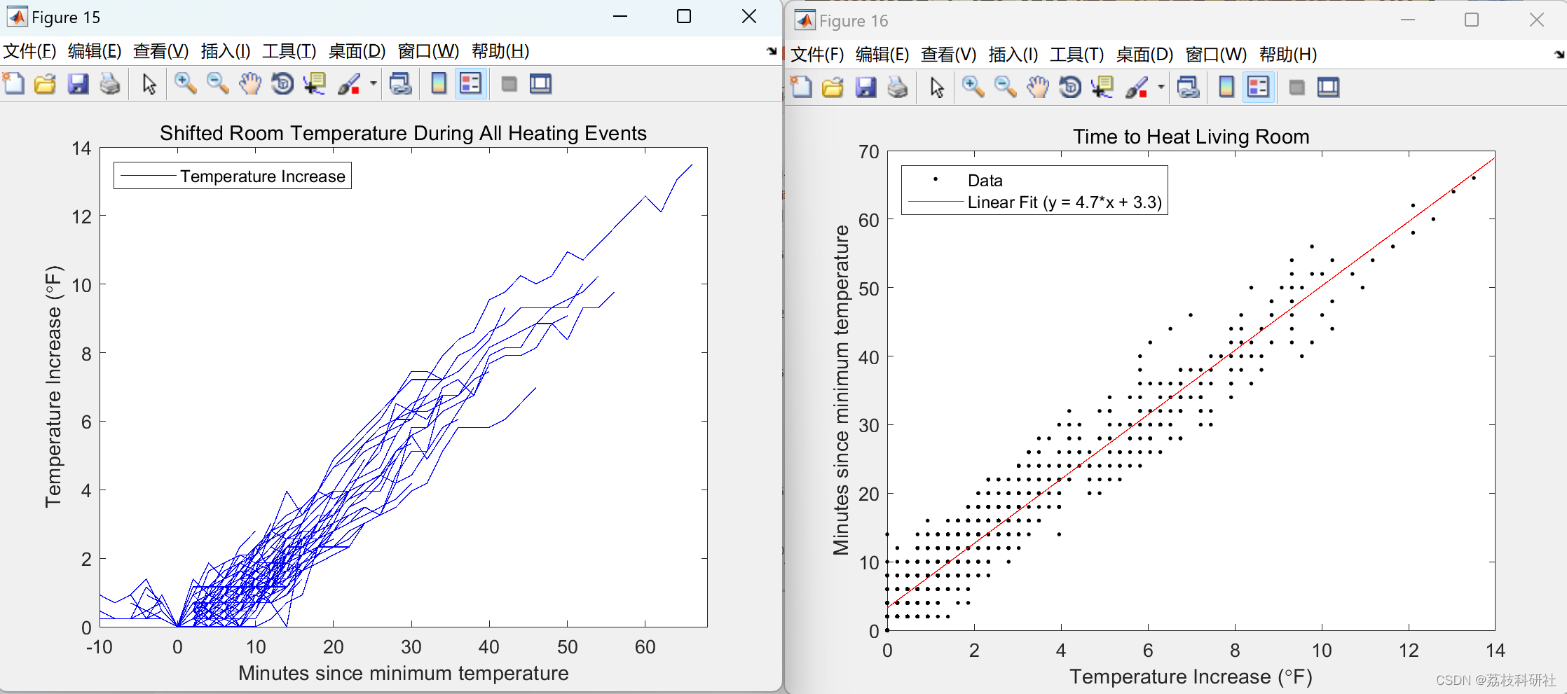
% Now let me fit a line to the data so I can get an equation for the time
% it takes to heat the living room.

%%
% First I collect all the time and temperature data into a single column
% vector and remove |NaN| values.

allTimes = segmentTimesShifted(:);
allTemps = segmentTempsShifted(:);
allTimes(isnan(allTemps)) = [];
allTemps(isnan(allTemps)) = [];

%%
% Then I can fit a line to the data.
linfit = polyfit(allTemps,allTimes,1);

%%
% Let's see how well we fit the data.

hold on
h2 = plot(xlim,polyval(linfit,xlim),'r-');
linfitstr = sprintf('Linear Fit (y = %.1f*x + %.1f)',linfit(1),linfit(2));
legend([ h1(1), h2(1) ],{'Data',linfitstr},'Location','NorthWest')

%%
% _Figure 18: The time it takes to heat the living room along with a linear fit to the data._
%
% Not a bad fit. Looking closer at the coefficients from the linear fit, it
% looks like it takes about 3 minutes after the radiators start to heat up
% for the room to start to warm up. After that, it takes about 5 minutes
% for each degree of temperature increase.

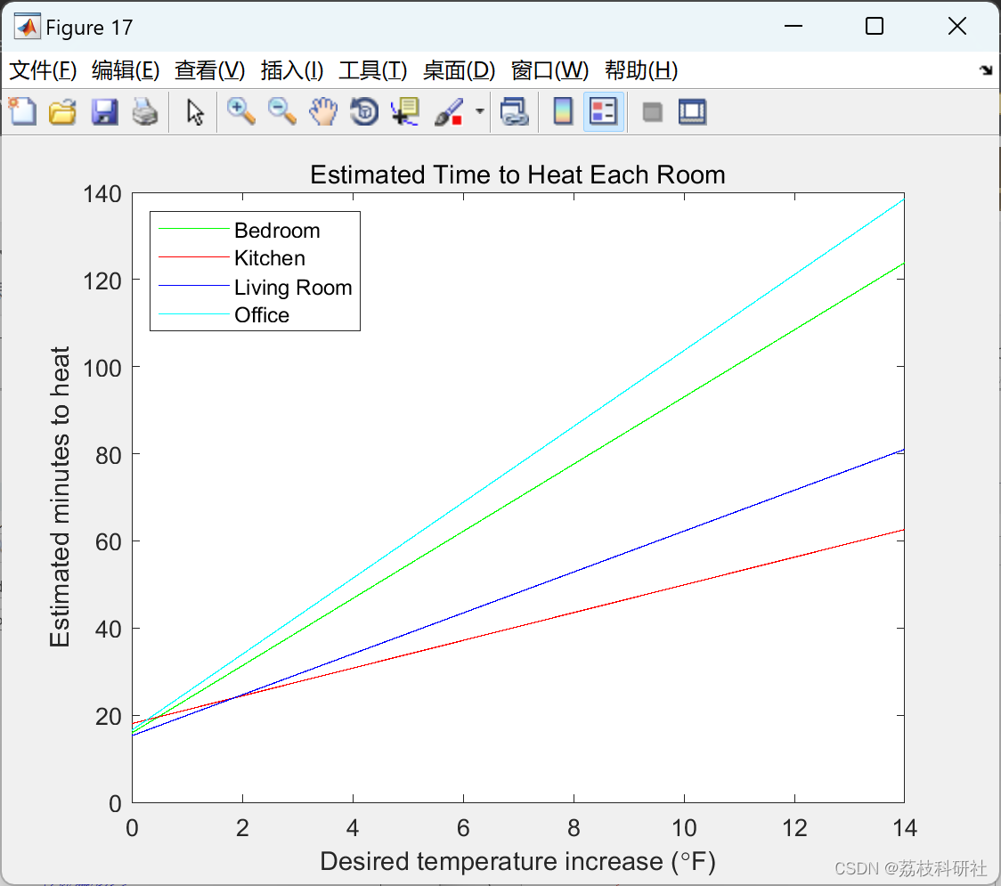
%% What room takes the longest to warm up?
% I can apply the techniques above to each room to find out how long each
% room takes to warm up. I took the code above and put it into a separate
% function called <../temperatureAnalysis.m |temperatureAnalysis|>, and
% applied that to each inside temperature sensor.

inside = [1 5 9 12];

figure
xl = [0 14];
for s = 1:size(inside,2)
linfits(s,1:2) = temperatureAnalysis(tempF(:,inside(s)), heaton, heatoff);
y = polyval(linfits(s,1:2),xl) + heatondelay;
plot(xl, y, lineSpecs{inside(s),1}, 'Color',lineSpecs{inside(s),2},...
'DisplayName',location{inside(s)})
hold on
end
legend('Location','NorthWest')
xlabel('Desired temperature increase (\circF)')
ylabel('Estimated minutes to heat')
title('Estimated Time to Heat Each Room')

%%
% _Figure 19: The estimated time it takes to heat each room in my apartment._