Tensorflow中文手册
介绍TensorFlow_w3cschool
模型结构图:
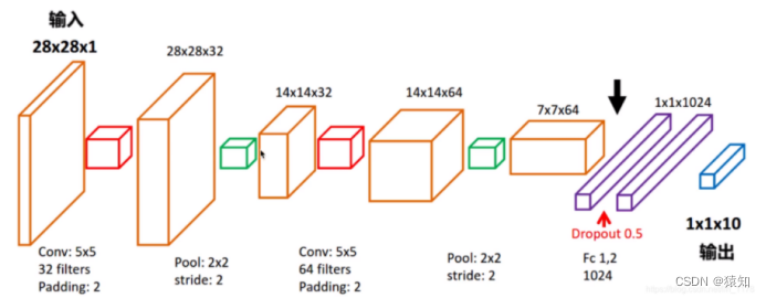
首先明确模型的输入及输出(先不考虑batch)
输入:一张手写数字图(28x28x1像素矩阵) 1是通道数
输出:预测的数字(1x10的one-hot向量)
one hot编码是将类别变量转换为机器学习算法易于利用的一种形式的过程,比如
输出[0,0,0,0,0,0,0,0,1,0]代表数字“8”
各层的维度说明(先不考虑batch)
输入层(28 x28 x1)
卷积层1的输出(28x28x32)(32 filters)
pooling层1的输出(14x14x32)
卷积层2的输出(14x14x64)(64 filters)
pooling层2的输出(7x7x64)
全连接层1的输出(1x1024)
全连接层2 含softmax的输出(1x10)
注意,训练时采用batch,只是加了一个维度而已,比如(28x28x1)→(100x28x28x1) batch=100
详细代码讲解
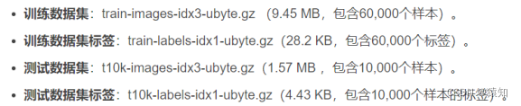
下载mnist手写数字图片数据集:
from tensorflow.examples.tutorials.mnist import input_data
mnist = input_data.read_data_sets('MNIST_data', one_hot=True)
若报错可自行前往
MNIST handwritten digit database, Yann LeCun, Corinna Cortes and Chris Burges
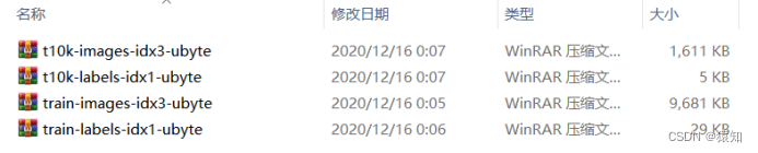
下载(或者其他地址),只要将四个压缩文件都放进MNIST_data文件夹即可,包含了四个部分:
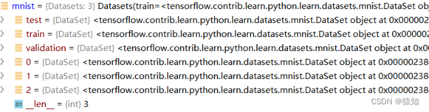
Tensorflow读取的mnist的数据形式(Datasets)
原训练集分出了5000作为验证集(实验中未使用)
训练集(train\0)的数量:55000
验证集(validation\1)的数量:5000
测试集(test\2)的数量:10000

补充:可视化train数据集图片
from tensorflow.examples.tutorials.mnist import input_data
import numpy as np
import matplotlib.pyplot as plt
plt.rcParams['font.sans-serif']=['SimHei'] #用来正常显示中文标签
plt.rcParams['axes.unicode_minus']=False
mnist = input_data.read_data_sets('MNIST_data', one_hot=True)
train_img = mnist.train.images
train_label = mnist.train.labels
for i in range(5):
img = np.reshape(train_img[i, :], (28, 28))
label = np.argmax(train_label[i, :])
plt.matshow(img, cmap = plt.get_cmap('gray'))
plt.title('第%d张图片 标签为%d' %(i+1,label))
plt.show()

卷积层1代码:
## conv1 layer 含pool ##
W_conv1 = weight_variable([5, 5, 1, 32])
# 初始化W_conv1为[5,5,1,32]的张量tensor,表示卷积核大小为5*5,1表示图像通道数(输入),32表示卷积核个数即输出32个特征图(即下一层的输入通道数)
# 张量说明:
# 3 这个 0 阶张量就是标量,shape=[]
# [1., 2., 3.] 这个 1 阶张量就是向量,shape=[3]
# [[1., 2., 3.], [4., 5., 6.]] 这个 2 阶张量就是二维数组,shape=[2, 3]
# [[[1., 2., 3.]], [[7., 8., 9.]]] 这个 3 阶张量就是三维数组,shape=[2, 1, 3]
# 即有几层中括号
b_conv1 = bias_variable([32])
# 偏置项,参与conv2d中的加法,维度会自动扩展到28x28x32(广播)
h_conv1 = tf.nn.relu(conv2d(x_image, W_conv1) + b_conv1)
# output size 28x28x32
h_pool1 = max_pool_2x2(h_conv1) # output size 14x14x32 卷积操作使用padding保持维度不变,只靠pool降维
其中:
xs = tf.placeholder(tf.float32, [None, 784], name='x_input')
ys = tf.placeholder(tf.float32, [None, 10], name='y_input')
x_image = tf.reshape(xs, [-1, 28, 28, 1])
# 创建两个占位符,xs为输入网络的图像,ys为输入网络的图像标签
# 输入xs(二维张量,shape为[batch, 784])变成4d的x_image,x_image的shape应该是[batch,28,28,1],第四维是通道数1
# -1表示自动推测这个维度的size
# reshape成了conv2d需要的输入形式;若是直接进入全连接层,则没必要reshape
——————————————以上使用到的函数的定义——————————————
注意:tensorflow的变量必须定义为tf.Variable类型
def weight_variable(shape):
# tf.truncated_normal从截断的正态分布中输出随机值.
initial = tf.truncated_normal(shape, stddev=0.1)
return tf.Variable(initial)
def bias_variable(shape):
initial = tf.constant(0.1, shape=shape)
return tf.Variable(initial)
def conv2d(x, W):
return tf.nn.conv2d(x, W, strides=[1, 1, 1, 1], padding='SAME')
# 卷积核移动步长为1,填充padding类型为SAME,可以不丢弃任何像素点, VALID丢弃边缘像素点
# 计算给定的4-D input和filter张量的2-D卷积
# input shape [batch, in_height, in_width, in_channels]
# filter shape [filter_height, filter_width, in_channels, out_channels]
# stride对应在这四维上的步长,默认[1,x,y,1]
def max_pool_2x2(x):
# 采用最大池化,也就是取窗口中的最大值作为结果
# x 是一个4维张量,shape为[batch,height,width,channels]
# ksize表示pool窗口大小为2x2,也就是高2,宽2
# strides,表示在height和width维度上的步长都为2
return tf.nn.max_pool(x, ksize=[1, 2, 2, 1], strides=[1, 2, 2, 1], padding='SAME')
———————————————————————————————————————
卷积层2代码:
## conv2 layer 含pool##
W_conv2 = weight_variable([5, 5, 32, 64]) # 同conv1,不过卷积核数增为64
b_conv2 = bias_variable([64])
h_conv2 = tf.nn.relu(conv2d(h_pool1, W_conv2) + b_conv2)
# output size 14x14x64
h_pool2 = max_pool_2x2(h_conv2)
# output size 7x7x64
全连接层1代码:
## fc1 layer ##
# 含1024个神经元,初始化(3136,1024)的tensor
W_fc1 = weight_variable([7 * 7 * 64, 1024])
b_fc1 = bias_variable([1024])
h_pool2_flat = tf.reshape(h_pool2, [-1, 7 * 7 * 64])
# 将conv2的输出reshape成[batch, 7*7*16]的张量,方便全连接层处理
h_fc1 = tf.nn.relu(tf.matmul(h_pool2_flat, W_fc1) + b_fc1)
h_fc1_drop = tf.nn.dropout(h_fc1, keep_prob)
其中:
xs = tf.placeholder(tf.float32, [None, 784], name='x_input')
ys = tf.placeholder(tf.float32, [None, 10], name='y_input')
keep_prob = tf.placeholder(tf.float32)
x_image = tf.reshape(xs, [-1, 28, 28, 1])
keep_prob_rate = 0.5
# 在机器学习的模型中,如果模型的参数太多,而训练样本又太少,训练出来的模型很容易产生过拟合的现象。
# 在训练神经网络的时候经常会遇到过拟合的问题,过拟合具体表现在:模型在训练数据上损失函数较小,预测准确率较高;但是在测试数据上损失函数比较大,预测准确率较低。
# 神经元按1-keep_prob概率置0,否则以1/keep_prob的比例缩放该元(并非保持不变)
# 这是为了保证神经元输出激活值的期望值与不使用dropout时一致,结合概率论的知识来具体看一下:假设一个神经元的输出激活值为a,在不使用dropout的情况下,其输出期望值为a,如果使用了dropout,神经元就可能有保留和关闭两种状态,把它看作一个离散型随机变量,符合概率论中的0-1分布,其输出激活值的期望变为 p*a+(1-p)*0=pa,为了保持测试集与训练集神经元输出的分布一致,可以在训练时除以此系数或者测试时乘以此系数,或者在测试时乘以该系数
全连接层2代码:
## fc2 layer 含softmax层##
# 含10个神经元,初始化(1024,10)的tensor
W_fc2 = weight_variable([1024, 10])
b_fc2 = bias_variable([10])
prediction = tf.nn.softmax(tf.matmul(h_fc1_drop, W_fc2) + b_fc2)
# 交叉熵函数
![]()
cross_entropy = tf.reduce_mean(-tf.reduce_sum(ys * tf.log(prediction),
reduction_indices=[1]))
补充tf.reduce_mean

计算张量的(各个维度上)元素的平均值,例如
x = tf.constant([[1., 1.], [2., 2.]])
tf.reduce_mean(x) # 1.5
tf.reduce_mean(x, 0) # [1.5, 1.5]
tf.reduce_mean(x, 1) # [1., 2.]T
0代表输出是个行向量,那么就是各行每个维度取mean
# 使用ADAM优化器来做梯度下降,学习率learning_rate=0.0001
learning_rate = 1e-4
train_step = tf.train.AdamOptimizer(learning_rate).minimize(cross_entropy)
# 模型训练后,计算测试集准确率
def compute_accuracy(v_xs, v_ys):
global prediction
# y_pre将v_xs(test)输入模型后得到的预测值 (10000,10)
y_pre = sess.run(prediction, feed_dict={xs: v_xs, keep_prob: 1})
# argmax(axis) axis = 1 返回结果为:数组中每一行最大值所在“列”索引值
# tf.equal返回布尔值,correct_prediction (10000,1)
correct_prediction = tf.equal(tf.argmax(y_pre, 1), tf.argmax(v_ys, 1))
# tf.cast将bool转成float32, tf.reduce_mean求均值,作为accuracy值(0到1)
accuracy = tf.reduce_mean(tf.cast(correct_prediction, tf.float32))
result = sess.run(accuracy, feed_dict={xs: v_xs, ys: v_ys, keep_prob: 1})
return result
TensorFlow 程序通常被组织成一个构建阶段(graph)和一个执行阶段.
上述阶段就是构建阶段,现在进入执行阶段,反复执行图中的训练操作,首先需要创建一个Session对象,如
sess = tf.Session() ****** sess.close()
Session对象在使用完后需要关闭以释放资源. 除了显式调用 close 外, 也可以使用 "with" 代码块 来自动完成关闭动作,如下
with tf.Session() as sess:
# 初始化图中所有Variables
init = tf.global_variables_initializer()
sess.run(init)
# 总迭代次数(batch)为max_epoch=1000,每次取100张图做batch梯度下降
for i in range(max_epoch):
# mnist.train.next_batch 默认shuffle=True,随机读取,batch大小为100
batch_xs, batch_ys = mnist.train.next_batch(100)
# 此batch是个2维tuple,batch[0]是(100,784)的样本数据数组,batch[1]是(100,10)的样本标签数组,分别赋值给batch_xs, batch_ys
sess.run(train_step, feed_dict={xs: batch_xs, ys: batch_ys, keep_prob: keep_prob})
# 暂时不进行赋值的元素叫占位符(如xs、ys),run需要它们时得赋值,feed_dict就是用来赋值的,格式为字典型
if (i+1) % 50 == 0:
print("step %d, test accuracy %g" % (i+1, compute_accuracy(
mnist.test.images, mnist.test.labels)))
利用自带的tensorboard可视化模型(深入理解图的概念)
tensorboard支持8种可视化,也就是上图中的8个选项卡,它们分别是:
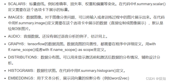
tensorboard通过运行一个本地服务器,监听6006端口,在浏览器发出请求时,分析训练时记录的数据,绘制训练过程中的数据曲线、图像。
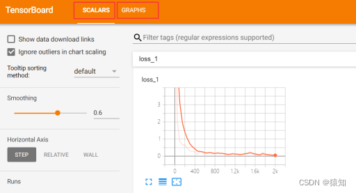

以可视化loss(scalars)、graphs为例:
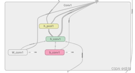
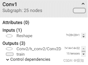
为了在graphs中展示节点名称,在设计网络时可用with tf.name_scope()限定命名空间
以第一个卷积层为例:
with tf.name_scope('Conv1'):
with tf.name_scope('W_conv1'):
W_conv1 = weight_variable([5, 5, 1, 32])
with tf.name_scope('b_conv1'):
b_conv1 = bias_variable([32])
with tf.name_scope('h_conv1'):
h_conv1 = tf.nn.relu(conv2d(x_image, W_conv1) + b_conv1)
with tf.name_scope('h_pool1'):
h_pool1 = max_pool_2x2(h_conv1)
同样地,对所有节点进行命名
如下,Conv1中的名称即命名结果
with tf.name_scope('loss'):
cross_entropy = tf.reduce_mean(-tf.reduce_sum(ys * tf.log(prediction),
reduction_indices=[1]))
在with tf.Session() as sess中添加
losssum = tf.summary.scalar('loss', cross_entropy)
# loss计入summary中,可以被统计
writer = tf.summary.FileWriter("", graph=sess.graph)
# tf.summary.FileWriter指定一个文件用来保存图
在if i % 50 == 0中添加
summery= sess.run(losssum, feed_dict={xs: batch_xs, ys: batch_ys, keep_prob: keep_prob_rate})
writer.add_summary(summery, i)
# add_summary()方法将训练过程数据保存在filewriter指定的文件中
在Terminal中输入
tensorboard --logdir=E:\cnn_mnist
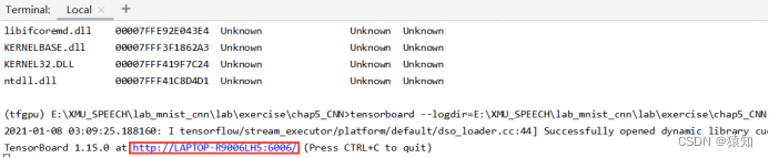
将网址中的LAPTOP-R9006LH5改为localhost,复制在浏览器中打开即可
附录(完整代码1):
import tensorflow as tf
from tensorflow.examples.tutorials.mnist import input_data
mnist = input_data.read_data_sets('MNIST_data', one_hot=True)
def weight_variable(shape):
# tf.truncated_normal从截断的正态分布中输出随机值.
initial = tf.truncated_normal(shape, stddev=0.1)
return tf.Variable(initial)
# 偏置初始化
def bias_variable(shape):
initial = tf.constant(0.1, shape=shape)
return tf.Variable(initial)
# 使用tf.nn.conv2d定义2维卷积
def conv2d(x, W):
# 卷积核移动步长为1,填充padding类型为SAME,简单地理解为以0填充边缘, VALID采用不填充的方式,多余地进行丢弃
# 计算给定的4-D input和filter张量的2-D卷积
# input shape [batch, in_height, in_width, in_channels]
# filter shape [filter_height, filter_width, in_channels, out_channels]
# stride 长度为4的1-D张量,input的每个维度的滑动窗口的步幅
return tf.nn.conv2d(x, W, strides=[1, 1, 1, 1], padding='SAME')
def max_pool_2x2(x):
# 采用最大池化,也就是取窗口中的最大值作为结果
# x 是一个4维张量,shape为[batch,height,width,channels]
# ksize表示pool窗口大小为2x2,也就是高2,宽2
# strides,表示在height和width维度上的步长都为2
return tf.nn.max_pool(x, ksize=[1, 2, 2, 1], strides=[1, 2, 2, 1], padding='SAME')
# 计算test set的accuracy,v_xs (10000,784), y_ys (10000,10)
def compute_accuracy(v_xs, v_ys):
global prediction
# y_pre将v_xs输入模型后得到的预测值 (10000,10)
y_pre = sess.run(prediction, feed_dict={xs: v_xs, keep_prob: 1})
# argmax(axis) axis = 1 返回结果为:数组中每一行最大值所在“列”索引值
# tf.equal返回布尔值,correct_prediction (10000,1)
correct_prediction = tf.equal(tf.argmax(y_pre, 1), tf.argmax(v_ys, 1))
# tf.cast将bool转成float32, tf.reduce_mean求均值,作为accuracy值(0到1)
accuracy = tf.reduce_mean(tf.cast(correct_prediction, tf.float32))
result = sess.run(accuracy, feed_dict={xs: v_xs, ys: v_ys, keep_prob: 1})
return result
xs = tf.placeholder(tf.float32, [None, 784], name='x_input')
ys = tf.placeholder(tf.float32, [None, 10], name='y_input')
max_epoch = 2000
keep_prob = tf.placeholder(tf.float32)
x_image = tf.reshape(xs, [-1, 28, 28, 1])
keep_prob_rate = 0
# 卷积层1
# input size 28x28x1 (以一个样本为例)batch=100 则100x28x28x1
W_conv1 = weight_variable([5, 5, 1, 32])
b_conv1 = bias_variable([32])
h_conv1 = tf.nn.relu(conv2d(x_image, W_conv1) + b_conv1)
# output size 28x28x32
h_pool1 = max_pool_2x2(h_conv1) # output size 14x14x32 卷积操作使用padding保持维度不变,只靠pool降维
# 卷积层2
W_conv2 = weight_variable([5, 5, 32, 64]) # 同conv1,不过卷积核数增为64
b_conv2 = bias_variable([64])
h_conv2 = tf.nn.relu(conv2d(h_pool1, W_conv2) + b_conv2)
# output size 14x14x64
h_pool2 = max_pool_2x2(h_conv2)
# output size 7x7x64
h_pool2_flat = tf.reshape(h_pool2, [-1, 7 * 7 * 64])
# 全连接层1
W_fc1 = weight_variable([7 * 7 * 64, 1024])
b_fc1 = bias_variable([1024])
# 将conv2的输出reshape成[batch, 7*7*16]的张量,方便全连接层处理
h_fc1 = tf.nn.relu(tf.matmul(h_pool2_flat, W_fc1) + b_fc1)
h_fc1_drop = tf.nn.dropout(h_fc1, keep_prob)
# 全连接层2
W_fc2 = weight_variable([1024, 10])
b_fc2 = bias_variable([10])
prediction = tf.nn.softmax(tf.matmul(h_fc1_drop, W_fc2) + b_fc2)
cross_entropy = tf.reduce_mean(-tf.reduce_sum(ys * tf.log(prediction),
reduction_indices=[1]))
learning_rate = 1e-4
train_step = tf.train.AdamOptimizer(learning_rate).minimize(cross_entropy)
with tf.Session() as sess:
# 初始化图中所有Variables
init = tf.global_variables_initializer()
sess.run(init)
# 总迭代次数(batch)为max_epoch=1000,每次取100张图做batch梯度下降
print("step 0, test accuracy %g" % (compute_accuracy(
mnist.test.images, mnist.test.labels)))
for i in range(max_epoch):
# mnist.train.next_batch 默认shuffle=True,随机读取,batch大小为100
batch_xs, batch_ys = mnist.train.next_batch(100)
# 此batch是个2维tuple,batch[0]是(100,784)的样本数据数组,batch[1]是(100,10)的样本标签数组,分别赋值给batch_xs, batch_ys
sess.run(train_step, feed_dict={xs: batch_xs, ys: batch_ys, keep_prob: keep_prob_rate})
# 暂时不进行赋值的元素叫占位符(如xs、ys),run需要它们时得赋值,feed_dict就是用来赋值的,格式为字典型
if (i + 1) % 50 == 0:
print("step %d, test accuracy %g" % (i + 1, compute_accuracy(
mnist.test.images, mnist.test.labels)))
附录(完整代码2 带tensorboad可视化):
import tensorflow.compat.v1 as tf
# import tensorflow as tf
from tensorflow.examples.tutorials.mnist import input_data
import os
# 导入input_data用于自动下载和安装MNIST数据集
mnist = input_data.read_data_sets('MNIST_data', one_hot=True)
learning_rate = 1e-4
keep_prob_rate = 0.7 # drop out比例(补偿系数)
# 为了保证神经元输出激活值的期望值与不使用dropout时一致,我们结合概率论的知识来具体看一下:假设一个神经元的输出激活值为a,
# 在不使用dropout的情况下,其输出期望值为a,如果使用了dropout,神经元就可能有保留和关闭两种状态,把它看作一个离散型随机变量,
# 它就符合概率论中的0-1分布,其输出激活值的期望变为 p*a+(1-p)*0=pa,为了保持测试集与训练集神经元输出的分布一致,可以训练时除以此系数或者测试时乘以此系数
# 即输出节点按照keep_prob概率置0,否则以1/keep_prob的比例缩放该节点(而并非保持不变)
max_epoch = 2000
# 权重矩阵初始化
def weight_variable(shape):
# tf.truncated_normal从截断的正态分布中输出随机值.
initial = tf.truncated_normal(shape, stddev=0.1)
return tf.Variable(initial)
# 偏置初始化
def bias_variable(shape):
initial = tf.constant(0.1, shape=shape)
return tf.Variable(initial)
# 使用tf.nn.conv2d定义2维卷积
def conv2d(x, W):
# 卷积核移动步长为1,填充padding类型为SAME,简单地理解为以0填充边缘, VALID采用不填充的方式,多余地进行丢弃
# 计算给定的4-D input和filter张量的2-D卷积
# input shape [batch, in_height, in_width, in_channels]
# filter shape [filter_height, filter_width, in_channels, out_channels]
# stride 长度为4的1-D张量,input的每个维度的滑动窗口的步幅
return tf.nn.conv2d(x, W, strides=[1, 1, 1, 1], padding='SAME')
def max_pool_2x2(x):
# 采用最大池化,也就是取窗口中的最大值作为结果
# x 是一个4维张量,shape为[batch,height,width,channels]
# ksize表示pool窗口大小为2x2,也就是高2,宽2
# strides,表示在height和width维度上的步长都为2
return tf.nn.max_pool(x, ksize=[1, 2, 2, 1], strides=[1, 2, 2, 1], padding='SAME')
# 计算test set的accuracy,v_xs (10000,784), y_ys (10000,10)
def compute_accuracy(v_xs, v_ys):
global prediction
# y_pre将v_xs输入模型后得到的预测值 (10000,10)
y_pre = sess.run(prediction, feed_dict={xs: v_xs, keep_prob: 1})
# argmax(axis) axis = 1 返回结果为:数组中每一行最大值所在“列”索引值
# tf.equal返回布尔值,correct_prediction (10000,1)
correct_prediction = tf.equal(tf.argmax(y_pre, 1), tf.argmax(v_ys, 1))
# tf.cast将bool转成float32, tf.reduce_mean求均值,作为accuracy值(0到1)
accuracy = tf.reduce_mean(tf.cast(correct_prediction, tf.float32))
result = sess.run(accuracy, feed_dict={xs: v_xs, ys: v_ys, keep_prob: 1})
return result
with tf.name_scope('input'):
xs = tf.placeholder(tf.float32, [None, 784], name='x_input')
ys = tf.placeholder(tf.float32, [None, 10], name='y_input')
keep_prob = tf.placeholder(tf.float32)
x_image = tf.reshape(xs, [-1, 28, 28, 1])
# 输入转化为4D数据,便于conv操作
# 把输入x(二维张量,shape为[batch, 784])变成4d的x_image,x_image的shape应该是[batch,28,28,1],第四维是通道数1
# -1表示自动推测这个维度的size
## conv1 layer ##
with tf.name_scope('Conv1'):
with tf.name_scope('W_conv1'):
W_conv1 = weight_variable([5, 5, 1, 32])
# 初始化W_conv1为[5,5,1,32]的张量tensor,表示卷积核大小为5*5,1表示图像通道数,6表示卷积核个数即输出6个特征图
# 3 这个 0 阶张量就是标量,shape=[]
# [1., 2., 3.] 这个 1 阶张量就是向量,shape=[3]
# [[1., 2., 3.], [4., 5., 6.]] 这个 2 阶张量就是二维数组,shape=[2, 3]
# [[[1., 2., 3.]], [[7., 8., 9.]]] 这个 3 阶张量就是三维数组,shape=[2, 1, 3]
# 即有几层中括号
with tf.name_scope('b_conv1'):
b_conv1 = bias_variable([32])
with tf.name_scope('h_conv1'):
h_conv1 = tf.nn.relu(conv2d(x_image, W_conv1) + b_conv1) # output size 28x28x32 5x5x1的卷积核作用在28x28x1的二维图上
with tf.name_scope('h_pool1'):
h_pool1 = max_pool_2x2(h_conv1) # output size 14x14x32 卷积操作使用padding保持维度不变,只靠pool降维
## conv2 layer ##
with tf.name_scope('Conv2'):
with tf.name_scope('W_conv2'):
W_conv2 = weight_variable([5, 5, 32, 64]) # patch 5x5, in size 32, out size 64
with tf.name_scope('b_conv2'):
b_conv2 = bias_variable([64])
with tf.name_scope('h_conv2'):
h_conv2 = tf.nn.relu(conv2d(h_pool1, W_conv2) + b_conv2) # output size 14x14x64
with tf.name_scope('h_pool2'):
h_pool2 = max_pool_2x2(h_conv2) # output size 7x7x64
# 全连接层 1
## fc1 layer ##
# 1024个神经元的全连接层
with tf.name_scope('Fc1'):
with tf.name_scope('W_fc1'):
W_fc1 = weight_variable([7 * 7 * 64, 1024])
with tf.name_scope('b_fc1'):
b_fc1 = bias_variable([1024])
with tf.name_scope('h_pool2_flat'):
h_pool2_flat = tf.reshape(h_pool2, [-1, 7 * 7 * 64])
with tf.name_scope('h_fc1'):
h_fc1 = tf.nn.relu(tf.matmul(h_pool2_flat, W_fc1) + b_fc1)
with tf.name_scope('h_fc1_drop'):
h_fc1_drop = tf.nn.dropout(h_fc1, keep_prob)
# 全连接层 2
## fc2 layer ##
with tf.name_scope('Fc2'):
with tf.name_scope('W_fc2'):
W_fc2 = weight_variable([1024, 10])
with tf.name_scope('b_fc2'):
b_fc2 = bias_variable([10])
with tf.name_scope('prediction'):
prediction = tf.nn.softmax(tf.matmul(h_fc1_drop, W_fc2) + b_fc2)
# 交叉熵函数
with tf.name_scope('loss'):
cross_entropy = tf.reduce_mean(-tf.reduce_sum(ys * tf.log(prediction),
reduction_indices=[1]))
# 使用ADAM优化器来做梯度下降,学习率为learning_rate0.0001
with tf.name_scope('train'):
train_step = tf.train.AdamOptimizer(learning_rate).minimize(cross_entropy)
with tf.Session() as sess:
# 初始化图中所有Variables
init = tf.global_variables_initializer()
sess.run(init)
losssum = tf.summary.scalar('loss', cross_entropy) # 若placeholde报错,则rerun
# merged = tf.summary.merge_all() # 只有loss值需要统计,故不需要merge
writer = tf.summary.FileWriter("", graph=sess.graph)
# tf.summary.FileWriter指定一个文件用来保存图
# writer.close()
# writer = tf.summary.FileWriter("", sess.graph) # 重新保存图时,要在console里rerun,否则graph会累计 cmd进入tfgpu环境 tensorboard --logdir=路径,将网址中的laptop替换为localhost
for i in range(max_epoch + 1):
# mnist.train.next_batch 默认shuffle=True,随机读取
batch_xs, batch_ys = mnist.train.next_batch(100)
# 此batch是个2维tuple,batch[0]是(100,784)的样本数据数组,batch[1]是(100,10)的样本标签数组
sess.run(train_step, feed_dict={xs: batch_xs, ys: batch_ys, keep_prob: keep_prob_rate})
if i % 50 == 0:
summery= sess.run(losssum, feed_dict={xs: batch_xs, ys: batch_ys, keep_prob: keep_prob_rate})
# summary = sess.run(merged, feed_dict={xs: batch_xs, ys: batch_ys, keep_prob: keep_prob_rate})
writer.add_summary(summery, i)
# add_summary()方法将训练过程数据保存在filewriter指定的文件中
print("step %d, test accuracy %g" % (i, compute_accuracy(
mnist.test.images, mnist.test.labels)))


![[league/glide]两行代码实现一套强大的图片处理HTTP服务](https://img-blog.csdnimg.cn/img_convert/274ee749364c64a712894fd10ec5ad7d.png)