最近给凯爹做的一个苦力活,统计检验这个东西说实话也挺有趣,跟算法设计一样,好的检验真的是挺难设计的,就有近似算法的那种感觉,检验很难保证size和power都很理想,所以就要做tradeoff,感觉这个假设检验的思路还是挺有趣,所以破例记录一下。
今天阳历生日(其实我每年都是过农历生日),凯爹职场情场皆得意,前脚拿到offer,后脚抱得美人归,说到底凯爹还是个挺励志的人,二战时吃那么多苦,如今终于是苦尽甘来(这不狠宰他一手哈哈哈哈哈哈哈哈
文章目录
- 假设检验① H 0 : A , B H_0:A,B H0:A,B是对角阵
- 1 生成模拟数据 X X X
- 2 虽然生成模拟数据时已知 A , B A,B A,B,但假设 A , B A,B A,B未知,对其进行估计。
- 2.1 第一种估计方法:Naive
- 2.2 第二种估计方法:Sample
- 2.3 第三种估计方法:Banded(只可对代表时间维度的矩阵 B B B使用)
- 3 对 A , B A,B A,B的估计值进行假设检验
- 4 上述1-3步骤,每组参数设置 { p , q , n , z } \{p,q,n,z\} {p,q,n,z}(共8种组合)重复1000次
- 4.1 对于每组参数设置,计算1000次试验后假设检验①的size
- 4.2 对于每组参数设置,计算1000次试验后假设检验①的power
- Appendix 代码实现
- 假设检验② H 0 : R A 1 = R A 2 H_0:R_A^1=R_A^2 H0:RA1=RA2
- 5 生成模拟数据 X X X
- 6 估计 B ~ ( g ) \tilde B^{(g)} B~(g)的3种方法
- 6.1 第一种估计方法:Naive
- 6.2 第二种估计方法:Sample
- 6.3 第三种估计方法:Banded
- 7 对两个协相关矩阵 A A A的相关系数矩阵 R A ( g ) R^{(g)}_A RA(g)进行假设检验
- 8 上述5-7步骤,每组参数设置 { p , q , n , z } \{p,q,n,z\} {p,q,n,z}(共8种组合),重复1000次
- 代码实现
假设检验① H 0 : A , B H_0:A,B H0:A,B是对角阵
1 生成模拟数据 X X X
对于matrix normal distribution, M N p q ( 0 , A , B ) MN_{pq}(0,A,B) MNpq(0,A,B), 0 0 0代表零均值, A , B A,B A,B分别是行与列的协方差。从分布中抽取两组模拟数据, X ( 1 ) = ( X 1 ( 1 ) , . . . , X n 1 ( 1 ) ) , X ( 2 ) = ( X 1 ( 2 ) , . . . , X n 2 ( 2 ) ) X^{(1)}=(X_1^{(1)},...,X_{n1}^{(1)}),X^{(2)}=(X_1^{(2)},...,X_{n2}^{(2)}) X(1)=(X1(1),...,Xn1(1)),X(2)=(X1(2),...,Xn2(2)), X 1 ( 1 ) X_1^{(1)} X1(1)维度为 p × q p\times q p×q。两组数据的分布中 A A A不一样, B B B一样, n 1 = n 2 = n n_1=n_2=n n1=n2=n
参数设置: p = { 10 , 20 } , q = { 10 , 20 } , n = { 5 , 8 } p=\{10,20\},q=\{10,20\},n=\{5,8\} p={10,20},q={10,20},n={5,8}
矩阵
A
p
×
p
=
A_{p\times p}=
Ap×p=
{
H
0
:
I
H
1
:
I
+
U
+
δ
I
1
+
δ
\left\{\begin{aligned} &H_0:I\\ &H_1:\frac{I+U+\delta I}{1+\delta} \end{aligned}\right.
⎩
⎨
⎧H0:IH1:1+δI+U+δI
矩阵 B q × q : b i j = 0. 4 ∣ i − j ∣ , 1 ≤ i , j ≤ q B_{q\times q}:b_{ij}=0.4^{|i-j|},1\le i,j\le q Bq×q:bij=0.4∣i−j∣,1≤i,j≤q
其中 δ = ∣ λ min ( I + U ) ∣ + 0.05 \delta=|\lambda_{\min}(I+U)|+0.05 δ=∣λmin(I+U)∣+0.05, λ min ( I + U ) \lambda_{\min}(I+U) λmin(I+U)表示取矩阵 I + U I+U I+U的最小特征根的绝对值。 U U U是稀疏对称矩阵,有 z = { 2 } z=\{2\} z={2}个非零元素。有 z 2 \frac z2 2z个非零元素在下/上三角中(不在对角线上),服从 U ( 2 ( log p n q ) 1 / 2 , 4 ( log p n q ) 1 / 2 ) U(2\left(\frac{\log p}{nq}\right)^{1/2},4\left(\frac{\log p}{nq}\right)^{1/2}) U(2(nqlogp)1/2,4(nqlogp)1/2)均匀分布,正负随机,位置随机。
2 虽然生成模拟数据时已知 A , B A,B A,B,但假设 A , B A,B A,B未知,对其进行估计。
对于每种估计方法,需要重复第3部分。
2.1 第一种估计方法:Naive
直接代入真实的 A , B A,B A,B
2.2 第二种估计方法:Sample
A p × p A_{p\times p} Ap×p的朴素估计: A ~ ∝ 1 n q ∑ k = 1 n X k X k ⊤ \tilde A\propto \frac{1}{nq}\sum_{k=1}^nX_kX_k^\top A~∝nq1∑k=1nXkXk⊤, B q × q B_{q\times q} Bq×q的朴素估计: B ~ ∝ 1 n p ∑ k = 1 n X k ⊤ X k \tilde B\propto \frac{1}{np}\sum_{k=1}^nX_k^\top X_k B~∝np1∑k=1nXk⊤Xk,注意,此处估计值差了常数倍,不可直接调用。
当
A
A
A已知时(用
A
~
\tilde A
A~代替),可以改进
B
B
B的估计:
B
^
=
1
n
p
∑
k
=
1
n
X
k
⊤
(
A
~
c
)
−
1
X
k
\widehat B=\frac1{np}\sum_{k=1}^nX_k^\top\left(\frac{\tilde A}{c}\right)^{-1}X_k
B
=np1k=1∑nXk⊤(cA~)−1Xk
c c c是一个未知常数,后续计算中会被抵消。
当
B
B
B已知时(用
B
~
\tilde B
B~代替),可以改进
A
A
A的估计:
A
^
=
1
n
q
∑
k
=
1
n
X
k
(
A
~
c
)
−
1
X
k
⊤
\widehat A=\frac1{nq}\sum_{k=1}^nX_k\left(\frac{\tilde A}{c}\right)^{-1}X_k^\top
A
=nq1k=1∑nXk(cA~)−1Xk⊤
c c c是一个未知常数,后续计算中会被抵消。
2.3 第三种估计方法:Banded(只可对代表时间维度的矩阵 B B B使用)
只保留
B
^
\widehat B
B
对角线以及两侧副对角线上的值:
B
ˉ
=
{
b
^
i
,
j
if
∣
i
−
j
∣
≤
2
0
otherwise
\bar B=\left\{\begin{aligned}&\hat b_{i,j}&&\text{if }|i-j|\le 2\\ &0&&\text{otherwise} \end{aligned}\right.
Bˉ={b^i,j0if ∣i−j∣≤2otherwise
3 对 A , B A,B A,B的估计值进行假设检验
3.1 假设检验① H 0 : B H_0:B H0:B是对角阵
记
M
n
=
max
1
≤
i
<
j
≤
q
M
i
j
,
M
i
j
M_n=\max_{1\le i<j\le q}M_{ij},M_{ij}
Mn=max1≤i<j≤qMij,Mij为
b
i
j
b_{ij}
bij标准化后的值,
M
i
j
=
b
^
i
j
2
θ
^
i
j
/
(
n
p
)
M_{ij}=\frac{\hat b_{ij}^2}{\hat \theta_{ij}/(np)}
Mij=θ^ij/(np)b^ij2,此处常数
c
c
c会相互抵消,其中:
θ
^
i
j
=
1
n
p
∑
k
=
1
n
∑
l
=
1
p
[
(
X
k
⊤
(
A
~
c
)
−
1
/
2
)
i
,
l
(
X
k
⊤
(
A
~
c
)
−
1
/
2
)
j
,
l
−
b
^
i
,
j
]
2
\hat \theta_{ij}=\frac1{np}\sum_{k=1}^n\sum_{l=1}^p\left[\left(X_k^\top\left(\frac{\tilde A}{c}\right)^{-1/2}\right)_{i,l}\left(X_k^\top\left(\frac{\tilde A}{c}\right)^{-1/2}\right)_{j,l}-\hat b_{i,j}\right]^2
θ^ij=np1k=1∑nl=1∑p
Xk⊤(cA~)−1/2
i,l
Xk⊤(cA~)−1/2
j,l−b^i,j
2
由于 M n − 4 log p + log log p M_n-4\log p+\log\log p Mn−4logp+loglogp服从Gumble分布,设统计量 Φ α = I ( M n ≥ α + 4 log q − log log q ) \Phi_\alpha=I(M_n\geq_{\alpha}+4\log q-\log\log q) Φα=I(Mn≥α+4logq−loglogq),其中 q α = − log ( 8 π ) − 2 log log ( 1 − α ) − 1 q_\alpha=-\log(8\pi)-2\log\log(1-\alpha)^{-1} qα=−log(8π)−2loglog(1−α)−1
当 Φ α = 1 \Phi_\alpha=1 Φα=1时拒绝 B B B是对角阵的原假设。
3.2 类似地,假设检验① H 0 : A H_0:A H0:A是对角阵
相当于转置 X ( 1 ) X^{(1)} X(1),再重复3.1操作,即,对应 p p p换成 q q q, X k ⊤ X_k^\top Xk⊤换成 X k X_k Xk, A ~ \tilde A A~换成 B ~ \tilde B B~
3.3 检验协方差 A A A哪些位置不为0
Ψ ( A ) = { ( i , j ) : a i , j ≠ 0 , 1 ≤ i < j ≤ p } Ψ ( τ = 4 ) = { ( i , j ) : M i , j ≥ τ p , 1 ≤ i < j ≤ p } \Psi(A)=\{(i,j):a_{i,j}\neq 0,1\le i<j\le p\}\\ \Psi(\tau=4)=\{(i,j):M_{i,j}\ge\tau p,1\le i<j\le p\} Ψ(A)={(i,j):ai,j=0,1≤i<j≤p}Ψ(τ=4)={(i,j):Mi,j≥τp,1≤i<j≤p}
3.4 检验协方差 B B B哪些位置不为0
Ψ ( B ) = { ( i , j ) : b i , j ≠ 0 , 1 ≤ i < j ≤ q } Ψ ( τ = 4 ) = { ( i , j ) : M i , j ≥ τ q , 1 ≤ i < j ≤ q } \Psi(B)=\{(i,j):b_{i,j}\neq 0,1\le i<j\le q\}\\ \Psi(\tau=4)=\{(i,j):M_{i,j}\ge\tau q,1\le i<j\le q\} Ψ(B)={(i,j):bi,j=0,1≤i<j≤q}Ψ(τ=4)={(i,j):Mi,j≥τq,1≤i<j≤q}
4 上述1-3步骤,每组参数设置 { p , q , n , z } \{p,q,n,z\} {p,q,n,z}(共8种组合)重复1000次
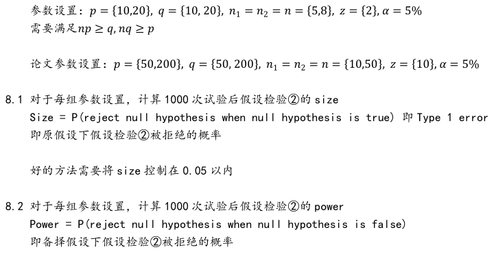
参数设置: p = { 10 , 20 } , q = { 10 , 20 } , n 1 = n 2 = n = { 5 , 8 } , z = { 2 } , α = 5 % p=\{10,20\},q=\{10,20\},n_1=n_2=n=\{5,8\},z=\{2\},\alpha=5\% p={10,20},q={10,20},n1=n2=n={5,8},z={2},α=5%,需要满足 n p ≥ q , n q ≥ p np\ge q,nq\ge p np≥q,nq≥p
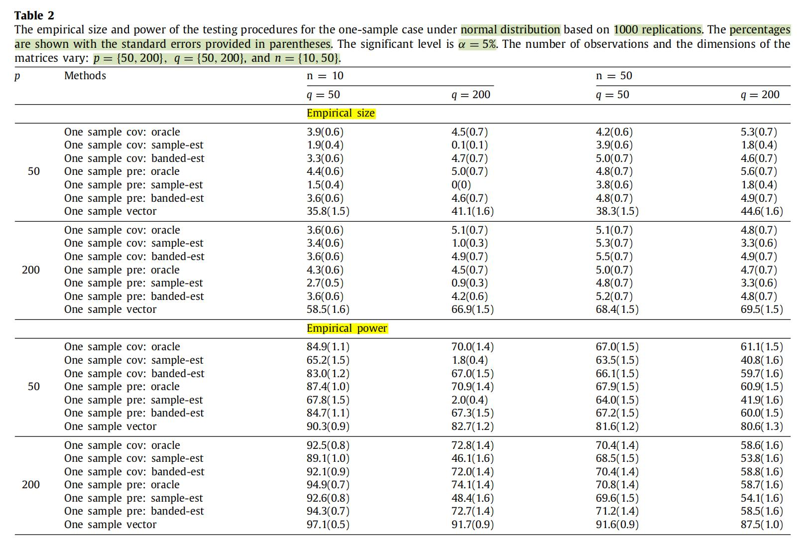
论文参数设置: p = { 50 , 200 } , q = { 50 , 200 } , n 1 = n 2 = n = { 10 , 50 } , z = { 8 } , α = 5 % p=\{50,200\},q=\{50,200\},n_1=n_2=n=\{10,50\},z=\{8\},\alpha=5\% p={50,200},q={50,200},n1=n2=n={10,50},z={8},α=5%
4.1 对于每组参数设置,计算1000次试验后假设检验①的size
Size=P(原假设为真,拒绝原假设)=P(犯第一类错误),即假设检验①种矩阵 A 0 A_0 A0被拒绝的概率,好的方法需要将size控制在0.05以内。
4.2 对于每组参数设置,计算1000次试验后假设检验①的power
Power=P(原假设为假,拒绝原假设),即假设检验①种 A 1 , B A_1,B A1,B被拒绝的概率。
Appendix 代码实现
这个仿真实现并不难,当然最好是用matlab写,这里给出numpy的示例代码。
-
矩阵正态分布随机变量的生成可以用scipy.stats里封装好的方法,也可以用cholesky分解来做。
-
测试结果表明小规模数据上的size还行,但是power明显不太好,但是原论文的效果就很漂亮:
- 但是这个量级的参数跑起来会特别慢。
# -*- coding: UTF-8 -*-
# @author: caoyang
# @email: caoyang@163.sufe.edu.cn

import math
import time
import numpy as np
from scipy.linalg import sqrtm
from scipy import stats

# Randomly generate matrix normal distributed matrix.
# M is a p-by-q matrix, U is a p-by-p matrix, and V is a q-by-q matrix.
def randomize_matrix_normal_variable(M, U, V):
	# X_rand = np.random.randn(*M.shape)
	# P = np.linalg.cholesky(U)
	# Q = np.linalg.cholesky(V)
	# return M + P @ X_rand @ Q.T
	return stats.matrix_normal(M, U, V).rvs()

# Randomly generate matrix U
def randomize_matrix_u(p, q, n, z=2):
	temp = np.sqrt((np.log(p) / n / q))
	low = 2 * temp
	high = 4 * temp
	U = np.zeros((p, p))	# initialize
	total_index = [(i, j) for i in range(p) for j in range(p)]
	np.random.shuffle(total_index)
	upper_index = []
	lower_index = []
	i = 0
	while len(upper_index) < int(z / 2) and len(lower_index) < int(z / 2):
		if total_index[i][0] < total_index[i][1] and len(upper_index) < int(z / 2):
			upper_index.append((total_index[i][0], total_index[i][1]))
			lower_index.append((total_index[i][1], total_index[i][0]))
		elif total_index[i][0] > total_index[i][1] and len(lower_index) < int(z / 2):
			lower_index.append((total_index[i][0], total_index[i][1]))
			upper_index.append((total_index[i][1], total_index[i][0]))
		i += 1
	for upper_indice, lower_indice in zip(upper_index, lower_index):
		sign = 2 * np.random.randint(0, 2) - 1	# random 1 and -1 for sign
		value = sign * np.random.uniform(low, high)
		U[upper_indice] = value
		U[lower_indice] = value
	return U

# Randomly generate matrix A
def randomize_matrix_a(hypothesis, p, q, n, z=2):
	if hypothesis == 0:
		return np.eye(p)
	elif hypothesis == 1:
		U = randomize_matrix_u(p, q, n, z)
		delta = abs(np.min(np.linalg.eigvals(np.eye(p) + U))) + .05
		return (np.eye(p) + U + delta * np.eye(p)) / (1 + delta)

	assert False, f'Hypothesis should be 0 or 1 but got {hypothesis} !'

# Randomly generate matrix B
def randomize_matrix_b(q):
	# return np.eye(q)
	return np.array([[0.4 ** (abs(i - j)) for j in range(q)] for i in range(q)])

# Calculate tilde A and tilde B
def calc_tilde_A_and_B(p, q, n, sample):
	tilde_A = np.zeros((p, p))
	for X in sample:
		tilde_A += X @ X.T
	tilde_A /= (n * q)
	tilde_B = np.zeros((q, q))
	for X in sample:
		tilde_B += X.T @ X
	tilde_B /= (n * p)
	return tilde_A, tilde_B

# Method 1
def estimate_method_1(A, B):
	hat_A = A
	hat_B = B
	return hat_A, hat_B

# Method 2
def estimate_method_2(p, q, n, sample):
	tilde_A, tilde_B = calc_tilde_A_and_B(p, q, n, sample)
	hat_A = np.zeros((p, p))
	for X in sample:
		hat_A += X @ np.linalg.inv(tilde_B) @ X.T
	hat_A /= (n * q)

	hat_B = np.zeros((q, q))
	for X in sample:
		hat_B += X.T @ np.linalg.inv(tilde_A) @ X
	hat_B /= (n * q)
	return hat_A, hat_B

# Method 3
def estimate_method_3(p, q, n, sample):
	hat_A, hat_B = estimate_method_2(p, q, n, sample)
	for i in range(p):
		for j in range(p):
			if abs(i - j) > 2:
				hat_B[i, j] = 0
	return hat_A, hat_B

# Hypothesis 1: B is diagonal matrix
def test_B(p, q, n, sample, tilde_A, hat_B, alpha=.05, tau=4):
	hat_theta = np.zeros((q, q))
	tilde_A_inv = sqrtm(np.linalg.inv(tilde_A))
	for i in range(q):
		for j in range(q):
			res = 0
			for k in range(n):
				X_k_tilde_A_inv = sample[k].T @ tilde_A_inv
				for l in range(p):
					res += (X_k_tilde_A_inv[i, l] * X_k_tilde_A_inv[j, l] - hat_B[i, j]) ** 2
			hat_theta[i, j] = res
	hat_theta /= (n * p)
	M = n * p * hat_B * hat_B / (hat_theta)
	for i in range(q):
		for j in range(i + 1):
			M[i, i] = -999
	M_n = np.max(M)
	q_alpha = -np.log(8 * math.pi) - 2 * np.log(-np.log(1 - alpha))
	Phi_alpha = 1 * (M_n > q_alpha + 4 * np.log(q) - np.log(np.log(q)))

	return Phi_alpha, M

# Hypothesis 2: A is diagonal matrix
def test_A(p, q, n, sample, tilde_B, hat_A, alpha=.05, tau=4):
	sample = list(map(lambda X: X.T, sample))
	return test_B(q, p, n, sample, tilde_B, hat_A, alpha)

def run():
	p_choices = [10, 20]
	q_choices = [10, 20]
	n_choices = [5, 8]
	# p_choices = [50, 200]
	# q_choices = [50, 200]
	# n_choices = [10, 50]
	N = 1000
	alpha = .05
	z = 2
	tau = 4

	time_string = time.strftime('%Y%m%d%H%M%S')
	filename = f'res1-{time_string}.txt'
	with open(filename, 'w') as f:
		pass

	for p in p_choices:
		for q in q_choices:
			for n in n_choices:
				print(f'p = {p}, q = {q}, n = {n}')
				count_Phi_alpha_B_0 = 0
				count_Phi_alpha_A_0 = 0
				count_Phi_alpha_B_1 = 0
				count_Phi_alpha_A_1 = 0
				for _ in range(N):
					A_0 = randomize_matrix_a(0, p, q, n, z)
					A_1 = randomize_matrix_a(1, p, q, n, z)
					B = randomize_matrix_b(q)

					sample_0 = [randomize_matrix_normal_variable(np.zeros((p, q)), A_0, B) for _ in range(n)]
					sample_1 = [randomize_matrix_normal_variable(np.zeros((p, q)), A_1, B) for _ in range(n)]

					tilde_A_0, tilde_B_0 = calc_tilde_A_and_B(p, q, n, sample_0)
					tilde_A_1, tilde_B_1 = calc_tilde_A_and_B(p, q, n, sample_0)

					hat_A_0, hat_B_0 = estimate_method_2(p, q, n, sample_0)
					hat_A_1, hat_B_1 = estimate_method_2(p, q, n, sample_1)
					# hat_A_0, hat_B_0 = estimate_method_1(A_0, B)
					# hat_A_1, hat_B_1 = estimate_method_1(A_1, B)

					Phi_alpha_B_0, M_B0 = test_B(p, q, n, sample_0, tilde_A_0, hat_B_0, alpha, tau)
					Phi_alpha_A_0, M_A0 = test_A(p, q, n, sample_0, tilde_B_0, hat_A_0, alpha, tau)
					Phi_alpha_B_1, M_B1 = test_B(p, q, n, sample_1, tilde_A_1, hat_B_1, alpha, tau)
					Phi_alpha_A_1, M_A1 = test_A(p, q, n, sample_1, tilde_B_1, hat_A_1, alpha, tau)

					count_Phi_alpha_B_0 += Phi_alpha_B_0
					count_Phi_alpha_A_0 += Phi_alpha_A_0
					count_Phi_alpha_B_1 += Phi_alpha_B_1
					count_Phi_alpha_A_1 += Phi_alpha_A_1

					#####################################
					# 3.3 & 3.4
					Psi_B0 = (B != 0) * 1												# 得到零一矩阵(可用于画热力图)
					Psi_tau_B0 = (M_B0 >= tau * p) * 1									# 得到零一矩阵(可用于画热力图)

					where_B0 = np.where(Psi_B0 == 1)
					print([(x, y) for (x, y) in zip(where_B0[0], where_B0[1])])			# 得到零一矩阵中元素1的坐标

					where_tau_B0 = np.where(Psi_tau_B0 == 1)
					print([(x, y) for (x, y) in zip(where_tau_B0[0], where_tau_B0[1])])	# 得到零一矩阵中元素1的坐标


					# ----------------------------------

					Psi_A0 = (A_0 != 0) * 1												# 得到零一矩阵(可用于画热力图)
					Psi_tau_A0 = (M_A0 >= tau * q) * 1									# 得到零一矩阵(可用于画热力图)

					where_A0 = np.where(Psi_A0 == 1)
					print([(x, y) for (x, y) in zip(where_A0[0], where_A0[1])])			# 得到零一矩阵中元素1的坐标

					where_tau_A0 = np.where(Psi_tau_A0 == 1)
					print([(x, y) for (x, y) in zip(where_tau_A0[0], where_tau_A0[1])])	# 得到零一矩阵中元素1的坐标

					# ----------------------------------
					# 以下类似
					Psi_B1 = (B != 0) * 1
					Psi_tau_B1 = (M_B1 >= tau * p) * 1

					# ----------------------------------

					Psi_A1 = (A_1 != 0) * 1
					Psi_tau_A1 = (M_A1 >= tau * q) * 1
					#####################################


				print('Phi_alpha_B_0: ', count_Phi_alpha_B_0)
				print('Phi_alpha_A_0: ', count_Phi_alpha_A_0)
				print('Phi_alpha_B_1: ', count_Phi_alpha_B_1)
				print('Phi_alpha_A_1: ', count_Phi_alpha_A_1)

				with open(filename, 'a') as f:
					f.write(f'Phi_alpha_B_0: {count_Phi_alpha_B_0}\n')
					f.write(f'Phi_alpha_A_0: {count_Phi_alpha_A_0}\n')
					f.write(f'Phi_alpha_B_1: {count_Phi_alpha_B_1}\n')
					f.write(f'Phi_alpha_A_1: {count_Phi_alpha_A_1}\n')
run()
假设检验② H 0 : R A 1 = R A 2 H_0:R_A^1=R_A^2 H0:RA1=RA2
5 生成模拟数据 X X X
数据从matrix normal distribution, M N p q ( 0 , A ( g ) , B ( g ) ) MN_{pq}(0,A^{(g)},B^{(g)}) MNpq(0,A(g),B(g))中生成。 B ( g ) B^{(g)} B(g)为 A R ( 1 ) AR(1) AR(1)过程的自相关系数矩阵,系数为0.8和0.9.此处简化使用协方差矩阵 B q × q g : b i j = 0. 4 ∣ i − j ∣ , 1 ≤ i , j ≤ q B^{g}_{q\times q}:b_{ij}=0.4^{|i-j|},1\le i,j\le q Bq×qg:bij=0.4∣i−j∣,1≤i,j≤q的相关系数矩阵,同**1 生成模拟数据 X X X**中一样。
H 0 H_0 H0下, A ( 1 ) = A ( 2 ) = Σ ( 1 ) = D 1 / 2 Σ ∗ ( 1 ) D 1 / 2 A^{(1)}=A^{(2)}=\Sigma^{(1)}=D^{1/2}{\Sigma^*}^{(1)}D^{1/2} A(1)=A(2)=Σ(1)=D1/2Σ∗(1)D1/2,其中:
Σ ∗ ( 1 ) = ( σ i , j ∗ ( 1 ) ) = { 1 if i = j 0.5 if 5 ( k − 1 ) + 1 ≤ i ≠ j ≤ 5 k with k = 1 , . . . , p / 5 0 otherwise {\Sigma^*}^{(1)}=(\sigma_{i,j}^{*(1)})=\left\{\begin{aligned} &1&&\text{if }i=j\\ &0.5&&\text{if }5(k-1)+1\le i\neq j\le 5k\text{ with }k=1,...,p/5\\ &0&&\text{otherwise} \end{aligned}\right. Σ∗(1)=(σi,j∗(1))=⎩ ⎨ ⎧10.50if i=jif 5(k−1)+1≤i=j≤5k with k=1,...,p/5otherwise
即非零值集中在对角线附近, D D D为对焦矩阵, d i , i = U n i f ( 0.5 , 2.5 ) d_{i,i}=Unif(0.5,2.5) di,i=Unif(0.5,2.5)
H 1 H_1 H1下, ( A ( 1 ) ) − 1 = ( Σ ( 1 ) + δ I ) / ( 1 + δ ) (A^{(1)})^{-1}=(\Sigma^{(1)}+\delta I)/(1+\delta) (A(1))−1=(Σ(1)+δI)/(1+δ), ( A ( 2 ) ) − 1 = ( Σ ( 1 ) + U + δ I ) / ( 1 + δ ) (A^{(2)})^{-1}=(\Sigma^{(1)}+U+\delta I)/(1+\delta) (A(2))−1=(Σ(1)+U+δI)/(1+δ),两者相差一个稀疏矩阵 U U U,其中 δ = ∣ min { λ min ( Σ ( 1 ) ) , λ min ( Σ ( 1 ) + U ) } ∣ + 0.05 \delta=|\min\{\lambda_{\min}(\Sigma^{(1)}),\lambda_{\min}(\Sigma^{(1)}+U)\}|+0.05 δ=∣min{λmin(Σ(1)),λmin(Σ(1)+U)}∣+0.05。 U U U是稀疏对称矩阵,有 z = 2 z=2 z=2个非零元素,有 z / 2 z/2 z/2个非零元素在下/上三角中(不在对角线上),服从 U ( 3 ( log p n q ) 1 / 2 , 5 ( log p n q ) 1 / 2 ) U(3\left(\frac{\log p}{nq}\right)^{1/2},5\left(\frac{\log p}{nq}\right)^{1/2}) U(3(nqlogp)1/2,5(nqlogp)1/2)的均匀分布,正负随机,位置随机。
6 估计 B ~ ( g ) \tilde B^{(g)} B~(g)的3种方法
对于每种估计方法,需要重复第7部分
6.1 第一种估计方法:Naive
直接代入真实的 B ( g ) B^{(g)} B(g)
6.2 第二种估计方法:Sample
B ~ ( g ) = 1 n g p ∑ k = 1 n g ( X k ( g ) ) ⊤ X k ( g ) \tilde B^{(g)}=\frac{1}{n_gp}\sum_{k=1}^{n_g}(X_k^{(g)})^\top X_k^{(g)} B~(g)=ngp1k=1∑ng(Xk(g))⊤Xk(g)
6.3 第三种估计方法:Banded
只保留
B
~
(
g
)
\tilde B^{(g)}
B~(g)对角线以及两侧副对角线上的值:
B
ˉ
(
g
)
=
{
b
~
i
,
j
(
g
)
if
∣
i
−
j
∣
≤
2
0
otherwise
\bar B^{(g)}=\left\{\begin{aligned}&\tilde b_{i,j}^{(g)}&&\text{if }|i-j|\le 2\\&0&&\text{otherwise}\end{aligned}\right.
Bˉ(g)={b~i,j(g)0if ∣i−j∣≤2otherwise
7 对两个协相关矩阵 A A A的相关系数矩阵 R A ( g ) R^{(g)}_A RA(g)进行假设检验
7.1 假设检验② H 0 : R A 1 = R A 2 H_0:R_A^1=R_A^2 H0:RA1=RA2,即第一组和第二组的相关系数矩阵是否相同
公式太长,直接截图了:

7.2 检验相关系数矩阵 R A 1 R_A^1 RA1和 R A 2 R_A^2 RA2哪些位置不同
Ψ ∗ ( R A 1 , R A 2 ) = { ( i , j ) : r ^ i , j ( 1 ) ≠ r ^ i , j ( 2 ) , 1 ≤ i < j ≤ p } Ψ ∗ ( τ = 4 ) = { ( i , j ) : M i , j ∗ ≥ τ log ( p ) , 1 ≤ i < j ≤ p } \Psi^*(R_A^1,R_A^2)=\{(i,j):\hat r_{i,j}^{(1)}\neq \hat r_{i,j}^{(2)},1\le i<j\le p\}\\ \Psi^*(\tau=4)=\{(i,j):M_{i,j}^*\ge \tau \log (p),1\le i < j \le p\} Ψ∗(RA1,RA2)={(i,j):r^i,j(1)=r^i,j(2),1≤i<j≤p}Ψ∗(τ=4)={(i,j):Mi,j∗≥τlog(p),1≤i<j≤p}
8 上述5-7步骤,每组参数设置 { p , q , n , z } \{p,q,n,z\} {p,q,n,z}(共8种组合),重复1000次
代码实现
跟第一个检验的代码有很大的共通处,其实我看到第二个才知道这个检验在做什么事情,大概是自相关时间序列上的协方差和相关系数检验:
# -*- coding: UTF-8 -*-
# @author: caoyang
# @email: caoyang@163.sufe.edu.cn

import math
import time
import numpy as np
from scipy.linalg import sqrtm
from scipy import stats

# Randomly generate matrix normal distributed matrix.
# M is a p-by-q matrix, U is a p-by-p matrix, and V is a q-by-q matrix.
def randomize_matrix_normal_variable(M, U, V):
	return stats.matrix_normal(M, U, V).rvs()

# Randomly generate matrix U
def randomize_matrix_u(p, q, n, z=2):
	temp = np.sqrt((np.log(p) / n / q))
	low = 3 * temp
	high = 5 * temp
	U = np.zeros((p, p))	# initialize
	total_index = [(i, j) for i in range(p) for j in range(p)]
	np.random.shuffle(total_index)
	upper_index = []
	lower_index = []
	i = 0
	while len(upper_index) < int(z / 2) and len(lower_index) < int(z / 2):
		if total_index[i][0] < total_index[i][1] and len(upper_index) < int(z / 2):
			upper_index.append((total_index[i][0], total_index[i][1]))
			lower_index.append((total_index[i][1], total_index[i][0]))
		elif total_index[i][0] > total_index[i][1] and len(lower_index) < int(z / 2):
			lower_index.append((total_index[i][0], total_index[i][1]))
			upper_index.append((total_index[i][1], total_index[i][0]))
		i += 1
	for upper_indice, lower_indice in zip(upper_index, lower_index):
		sign = 2 * np.random.randint(0, 2) - 1	# random 1 and -1 for sign
		value = sign * np.random.uniform(low, high)
		U[upper_indice] = value
		U[lower_indice] = value
	return U

# Randomly generate matrix A
def randomize_matrix_a(hypothesis, p, q, n, z=2):
	Sigma_star = np.zeros((p, p))
	def _check(_i, _j):
		if _i == _j:
			return False
		for _k in range(p // 5):
			if 5 * (_k - 1) <= _i < 5 * _k and 5 * (_k - 1) <= _j < 5 * _k:
				return True
		return False
	for i in range(p):
		for j in range(p):
			if i == j:
				Sigma_star[i, j] = 1
			elif _check(i, j):
				Sigma_star[i, j] = .5
			else:
				Sigma_star[i, j] = 0

	D = np.diag(np.random.uniform(.5, 2.5, p))
	D_sqrt = np.sqrt(D)
	Sigma = D_sqrt @ Sigma_star @ D_sqrt

	if hypothesis == 0:
		A_1 = Sigma[:, :]
		A_2 = Sigma[:, :]
		return A_1, A_2


	elif hypothesis == 1:
		U = randomize_matrix_u(p, q, n, z)
		delta = abs(min(
			np.min(np.linalg.eigvals(Sigma + U)),
			np.min(np.linalg.eigvals(Sigma)),
		)) + .05
		A_1 = np.linalg.inv((Sigma + delta * np.eye(p)) / (1 + delta))
		A_2 = np.linalg.inv((Sigma + U + delta * np.eye(p)) / (1 + delta))
		# A_1 = (Sigma + delta * np.eye(p)) / (1 + delta)
		# A_2 = (Sigma + U + delta * np.eye(p)) / (1 + delta)
		return A_1, A_2

	assert False, f'Hypothesis should be 0 or 1 but got {hypothesis} !'


# Randomly generate matrix B
def randomize_matrix_b(q):
	# return np.eye(q)
	return np.array([[0.4 ** (abs(i - j)) for j in range(q)] for i in range(q)])

# Calculate tilde B
def calc_tilde_B(p, q, n, sample):
	tilde_B = np.zeros((q, q))
	for X in sample:
		tilde_B += X.T @ X
	tilde_B /= (n * p)
	return tilde_B


# Calculate hat A
def calc_hat_A(p, q, n, sample, tilde_B):
	hat_A = np.zeros((p, p))
	tilde_B_inv = np.linalg.inv(tilde_B)
	for X in sample:
		hat_A += X @ tilde_B_inv @ X.T
	hat_A /= (n * q)
	return hat_A

# Calculate hat R
def calc_hat_R(p, q, n, hat_A):
	hat_R = np.zeros((p, p))
	for i in range(p):
		for j in range(p):
			hat_R[i, j] = hat_A[i, j] / np.sqrt(hat_A[i, i] * hat_A[j, j])
	return hat_R


# Method 1
def estimate_method_1(B):
	hat_B = B
	return hat_B

# Method 2
def estimate_method_2(p, q, n, sample):
	tilde_B = calc_tilde_B(p, q, n, sample)
	return tilde_B

# Method 3
def estimate_method_3(p, q, n, sample):
	bar_B = calc_tilde_B(p, q, n, sample)
	for i in range(p):
		for j in range(p):
			if abs(i - j) > 2:
				bar_B[i, j] = 0
	return bar_B

# Hypothesis: R_A^1 = R_A^2
def test(p, q, n, A_1, A_2, B, sample_1, sample_2, alpha=0.05, tau=4):
	tilde_B_1 = calc_tilde_B(p, q, n, sample_1)
	tilde_B_2 = calc_tilde_B(p, q, n, sample_2)

	# 上面是用的estimate_method_2, 可以用另外两种
	# tilde_B_1 = estimate_method_1(B)
	# tilde_B_2 = estimate_method_1(B)
	# tilde_B_1 = estimate_method_2(p, q, n, sample_1)
	# tilde_B_2 = estimate_method_2(p, q, n, sample_2)
	# tilde_B_1 = estimate_method_3(p, q, n, sample_1)
	# tilde_B_2 = estimate_method_3(p, q, n, sample_2)

	hat_A_1 = calc_hat_A(p, q, n, sample_1, tilde_B_1)
	hat_A_2 = calc_hat_A(p, q, n, sample_2, tilde_B_2)
	hat_R_1 = calc_hat_R(p, q, n, hat_A_1)
	hat_R_2 = calc_hat_R(p, q, n, hat_A_2)

	tilde_B_1_inv = sqrtm(np.linalg.inv(tilde_B_1))
	tilde_B_2_inv = sqrtm(np.linalg.inv(tilde_B_2))

	M = np.zeros((p, p))
	for i in range(p):
		for j in range(p):
			theta_1 = 0
			theta_2 = 0
			for k in range(n):
				X_k_tilde_B_1_inv = sample_1[k] @ tilde_B_1_inv
				X_k_tilde_B_2_inv = sample_2[k] @ tilde_B_2_inv
				for l in range(q):
					theta_1 += (X_k_tilde_B_1_inv[i, l] * X_k_tilde_B_1_inv[j, l] - hat_A_1[i, j]) ** 2
					theta_2 += (X_k_tilde_B_2_inv[i, l] * X_k_tilde_B_2_inv[j, l] - hat_A_2[i, j]) ** 2
			theta_1 /= (n * q)
			theta_2 /= (n * q)
			pretty_theta_1 = theta_1 / hat_A_1[i, i] / hat_A_1[j, j]
			pretty_theta_2 = theta_2 / hat_A_2[i, i] / hat_A_2[j, j]
			M[i, j] = ((hat_R_1[i, j] - hat_R_2[i, j]) ** 2) / (pretty_theta_1 / n / q + pretty_theta_2 / n / q)

	for i in range(p):
		for j in range(i + 1):
			M[i, i] = -999

	M_n = np.max(M)
	q_alpha = -np.log(8 * math.pi) - 2 * np.log(-np.log(1 - alpha))
	Phi_alpha = 1 * (M_n > q_alpha + 4 * np.log(q) - np.log(np.log(q)))

	##########################
	# 7.2
	# ------------------------
	Psi_star = 1 * (hat_R_1 != hat_R_2)												# 得到零一矩阵(可用于画热力图)
	hat_Psi_star = 1 * (M > tau * np.log(p))										# 得到零一矩阵(可用于画热力图)

	where_Psi_star = np.where(Psi_star == 1)
	# print([(x, y) for (x, y) in zip(where_Psi_star[0], where_Psi_star[1])])			# 得到零一矩阵中元素1的坐标

	where_hat_Psi_star = np.where(hat_Psi_star == 1)
	# print([(x, y) for (x, y) in zip(where_hat_Psi_star[0], where_hat_Psi_star[1])])	# 得到零一矩阵中元素1的坐标
	##########################

	return Phi_alpha, Psi_star, hat_Psi_star

def run():
	p_choices = [10, 20]
	q_choices = [10, 20]
	n_choices = [5, 8]
	z = 2
	alpha = .05
	N = 1000
	tau = 4

	time_string = time.strftime('%Y%m%d%H%M%S')
	filename = f'res2-{time_string}.txt'
	with open(filename, 'w') as f:
		pass

	for p in p_choices:
		for q in q_choices:
			for n in n_choices:
				print(f'p = {p}, q = {q}, n = {n}')
				count_Phi_alpha_0 = 0
				count_Phi_alpha_1 = 0
				for _ in range(N):
					A_01, A_02 = randomize_matrix_a(0, p, q, n, z)
					A_11, A_12 = randomize_matrix_a(1, p, q, n, z)
					B = randomize_matrix_b(q)
					sample_01 = [randomize_matrix_normal_variable(np.zeros((p, q)), A_01, B) for _ in range(n)]
					sample_02 = [randomize_matrix_normal_variable(np.zeros((p, q)), A_02, B) for _ in range(n)]
					sample_11 = [randomize_matrix_normal_variable(np.zeros((p, q)), A_11, B) for _ in range(n)]
					sample_12 = [randomize_matrix_normal_variable(np.zeros((p, q)), A_12, B) for _ in range(n)]

					# 7.2的Psi在这里返回
					Phi_alpha_0, Psi_star_0, hat_Psi_star_0 = test(p, q, n, A_01, A_02, B, sample_01, sample_02, alpha, tau)
					Phi_alpha_1, Psi_star_1, hat_Psi_star_1 = test(p, q, n, A_11, A_12, B, sample_11, sample_12, alpha, tau)

					count_Phi_alpha_0 += Phi_alpha_0
					count_Phi_alpha_1 += Phi_alpha_1
				print('Phi_alpha_0: ', count_Phi_alpha_0)
				print('Phi_alpha_1: ', count_Phi_alpha_1)

				with open(filename, 'a') as f:
					f.write(f'Phi_alpha_0: {count_Phi_alpha_0}\n')
					f.write(f'Phi_alpha_1: {count_Phi_alpha_1}\n')


if __name__ == '__main__':

	run()