总结
参考
菜菜的sklearn课堂——随机森林
算法使用过程
#导入数据集模块
from sklearn import datasets
#分别加载iris和digits数据集
iris = datasets.load_iris() #鸢尾花数据集
# print(dir(datasets))
# print(iris_dataset.keys())
# dict_keys(['data', 'target', 'frame', 'target_names', 'DESCR', 'feature_names', 'filename', 'data_module'])
from sklearn.model_selection import train_test_split
X_train,X_test,y_train,y_test=train_test_split(iris.data,iris.target,test_size=0.4,random_state=0)
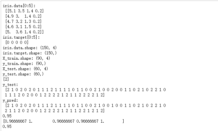
print("iris.data[0:5]:\n",iris.data[0:5])
print("iris.target[0:5]:\n",iris.target[0:5])
print("iris.data.shape:",iris.data.shape)
print("iris.target.shape:",iris.target.shape)
print("X_train.shape:",X_train.shape)
print("y_train.shape:",y_train.shape)
print("X_test.shape:",X_test.shape)
print("y_test.shape:",y_test.shape)
# 第二步使用sklearn模型的选择
from sklearn import svm
svc = svm.SVC(gamma='auto')
#第三步使用sklearn模型的训练
svc.fit(X_train, y_train)
# 第四步使用sklearn进行模型预测
print(svc.predict([[5.84,4.4,6.9,2.5]]))
#第五步机器学习评测的指标
#机器学习库sklearn中,我们使用metrics方法实现:
import numpy as np
from sklearn.metrics import accuracy_score
print("y_test:\n",y_test)
y_pred = svc.predict(X_test)
print("y_pred:\n",y_pred)
print(accuracy_score(y_test, y_pred))
#第五步机器学习评测方法:交叉验证 (Cross validation)
#机器学习库sklearn中,我们使用cross_val_score方法实现:
from sklearn.model_selection import cross_val_score
scores = cross_val_score(svc, iris.data, iris.target, cv=5)
print(scores)
#第六步机器学习:模型的保存
#机器学习库sklearn中,我们使用joblib方法实现:
# from sklearn.externals import joblib
import joblib
joblib.dump(svc, 'filename.pkl')
svc1 = joblib.load('filename.pkl')
#测试读取后的Model
print(svc1.score(X_test, y_test))
输出为:
集成学习
集成算法会考虑多个评估器的建模结果,汇总之后得到一个综合的结果,以此来获取比单个模型更好的回归或分类表现。
sklearn中的集成算法模块ensemble
| 类 | 类的功能 |
|---|---|
| ensemble.AdaBoostClassifier | AdaBoost分类 |
| ensemble.AdaBoostRegressor | Adaboost回归 |
| ensemble.BaggingClassifier | 装袋分类器 |
| ensemble.BaggingRegressor | 装袋回归器 |
| ensemble.ExtraTreesClassifier | Extra-trees分类(超树,极端随机树) |
| ensemble.ExtraTreesRegressor | Extra-trees回归 |
| ensemble.GradientBoostingClassifier | 梯度提升分类 |
| ensemble.GradientBoostingRegressor | 梯度提升回归 |
| ensemble.IsolationForest | 隔离森林 |
| ensemble.RandomForestClassifier | 随机森林分类 |
| ensemble.RandomForestRegressor | 随机森林回归 |
| ensemble.RandomTreesEmbedding | 完全随机树的集成 |
| ensemble.VotingClassifier | 用于不合适估算器的软投票/多数规则分类器 |
RandomForestClassifier
class sklearn.ensemble.RandomForestClassifier (n_estimators=’10’, criterion=’gini’, max_depth=None,
min_samples_split=2, min_samples_leaf=1, min_weight_fraction_leaf=0.0, max_features=’auto’,
max_leaf_nodes=None, min_impurity_decrease=0.0, min_impurity_split=None, bootstrap=True, oob_score=False,
n_jobs=None, random_state=None, verbose=0, warm_start=False, class_weight=None)
随机森林是非常具有代表性的Bagging集成算法,它的所有基评估器都是决策树,分类树组成的森林就叫做随机森林分类器,回归树所集成的森林就叫做随机森林回归器。这一节主要讲解RandomForestClassifier,随机森林分类器。
|
2.1 重要参数
2.1.1 控制基评估器的参数
| 参数 | 含义 |
|---|---|
| criterion | 不纯度的衡量指标,有基尼系数和信息熵两种选择 |
| max_depth | 树的最大深度,超过最大深度的树枝都会被剪掉 |
| min_samples_leaf | 一个节点在分枝后的每个子节点都必须包含至少min_samples_leaf个训练样本,否则分枝就不会发生 |
| min_samples_split | 一个节点必须要包含至少min_samples_split个训练样本,这个节点才允许被分枝,否则分枝就不会发生 |
| max_features | max_features限制分枝时考虑的特征个数,超过限制个数的特征都会被舍弃,默认值为总特征个数开平方取整 |
| min_impurity_decrease | 限制信息增益的大小,信息增益小于设定数值的分枝不会发生 |
2.1.2 n_estimators
这个参数是指随机森林中树的个数,对随机森林模型的精确性影响是单调的,n_estimators越大,模型的效果往往越好。但是相应的,任何模型都有决策边界,n_estimators达到一定的程度之后,随机森林的精确性往往不再上升或开始波动,并且,n_estimators越大,需要的计算量和内存也越大,训练的时间也会越来越长。所以这个参数要在训练难度和模型效果之间取得平衡。
n_estimators的默认值在现有版本的sklearn中是10,但是在即将更新的0.22版本中,这个默认值会被修正为100。这个修正显示出了使用者的调参倾向:要更大的n_estimators。一般来说,[0,200]间取值比较好。
2.2代码实现
# 针对红酒数据集,一个随机森林和单个决策树的效益对比
# 1.导入需要的包
# %matplotlib inline # 告诉python画图需要这个环境,
# 是IPython的魔法函数,可以在IPython编译器里直接使用,作用是内嵌画图,省略掉plt.show()这一步,直接显示图像。
# 如果不加这一句的话,我们在画图结束之后需要加上plt.show()才可以显示图像
from sklearn.tree import DecisionTreeClassifier # 导入决策树分类器
from sklearn.ensemble import RandomForestClassifier# 导入随机森林分类器
from sklearn.datasets import load_wine
from sklearn.model_selection import train_test_split
from sklearn.model_selection import cross_val_score# 交叉验证的包
import matplotlib.pyplot as plt# 画图用的
# 2.导入需要的数据集
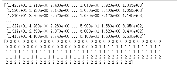
wine = load_wine()
print(wine.data) # wine是一个字典 (178,13)
print(wine.target)
输出为:
# 3.sklearn建模的基本流程
# 实例化
# 训练集代入实例化后的模型进行训练,使用的接口是fit
# 使用其它接口将测试集导入训练好的模型,获得结果(score,y_test)

Xtrain, Xtest, Ytrain, Ytest = train_test_split(wine.data, wine.target, test_size=0.3)
clf = DecisionTreeClassifier(random_state=0)# random_state控制树的生成模式,random_state=0让它只能生成一棵树
rfc = RandomForestClassifier(random_state=0)# random_state也是控制随机性的,但和决策树的有些许不同
clf = clf.fit(Xtrain, Ytrain)
rfc = rfc.fit(Xtrain, Ytrain)
score_c = clf.score(Xtest, Ytest)
score_r = rfc.score(Xtest, Ytest)
print('Single Tree:{}'.format(score_c)
      , 'Random Forest:{}'.format(score_r)# format后面()里的内容是放到前面{}里的
      )
输出为:

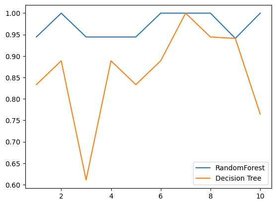
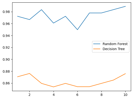
# 4.画出随机森林和决策树在一组交叉验证下的效果对比
# 复习交叉验证:将数据集划分为n份,依次取每一份做测试集,其余n-1份做训练集,多次训练模型以观测模型稳定性的方法
rfc = RandomForestClassifier(n_estimators=25)
rfc_s = cross_val_score(rfc, wine.data, wine.target, cv=10)
# 四个参数分别是:实例化好的模型,完整的特征矩阵,完整的标签,交叉验证的次数
clf = DecisionTreeClassifier()
clf_s = cross_val_score(clf, wine.data, wine.target, cv=10)
plt.plot(range(1, 11), rfc_s, label="RandomForest")
# 三个参数分别是:x的取值[1,11),y的取值,折线的标签
plt.plot(range(1, 11), clf_s, label="Decision Tree")
# 一个plot里面只能有一个标签,所以想显示折线的标签就只能写两行
plt.legend()# 显示图例
plt.show()# 展示图像
# ====================一种更加有趣也更简单的写法===================
"""
label = "RandomForest"
for model in [RandomForestClassifier(n_estimators=25),DecisionTreeClassifier()]:
    score = cross_val_score(model,wine.data,wine.target,cv=10)
    print("{}:".format(label)),print(score.mean())
    plt.plot(range(1,11),score,label = label)
    plt.legend()
    label = "DecisionTree"
"""
输出为:
# 5.画出随即森林和决策树在十组交叉验证下的效果对比(一般这部分不用做)
rfc_l = []
clf_l = []
for i in range(10):
    rfc = RandomForestClassifier(n_estimators=25)
    rfc_s = cross_val_score(rfc, wine.data, wine.target, cv=10).mean()
    rfc_l.append(rfc_s)
    clf = DecisionTreeClassifier()
    clf_s = cross_val_score(clf, wine.data, wine.target, cv=10).mean()
    clf_l.append(clf_s)

plt.plot(range(1, 11), rfc_l, label="Random Forest")
plt.plot(range(1, 11), clf_l, label="Decision Tree")
plt.legend()
plt.show()
# 是否有注意到,单个决策树的波动轨迹和随机森林一致?
# 再次验证了我们之前提到的,单个决策树的准确率越高,随机森林的准确率也会越高
输出为:
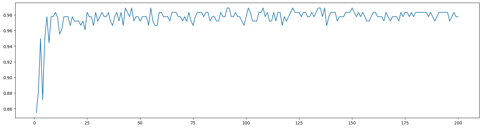
# 6.n_estimators的学习曲线
superpa = []
for i in range(200):
    rfc = RandomForestClassifier(n_estimators=i+1, n_jobs=-1) # 实例化
    rfc_s = cross_val_score(rfc, wine.data, wine.target, cv=10).mean() # 交叉验证
    superpa.append(rfc_s) # 将交叉验证的结果放到列表里
print(max(superpa), superpa.index(max(superpa))) # list.index(object)会返回对象object在列表list当中的索引
plt.figure(figsize=[20, 5])
plt.plot(range(1, 201), superpa)
plt.show()
输出为:
0.9888888888888889 42
模型融合
安装xgboost
!pip install xgboost
导入依赖
import sys
import os
print("Python version: {}". format(sys.version))
import pandas as pd # 加载csv等表格数据
print("pandas version: {}". format(pd.__version__))

import matplotlib # 画图
print("matplotlib version: {}". format(matplotlib.__version__))

import numpy as np #数据运算
print("NumPy version: {}". format(np.__version__))

import scipy as sp #高级数学运算
print("SciPy version: {}". format(sp.__version__))

import IPython
from IPython import display #美化DataFrame的输出


import sklearn #机器学习算法
print("scikit-learn version: {}". format(sklearn.__version__))

#基础库
import random
import time


#忽略警告
import warnings
warnings.filterwarnings('ignore')
print('-'*25)
输出为:
Python version: 3.6.3 |Anaconda custom (64-bit)| (default, Oct 15 2017, 03:27:45) [MSC v.1900 64 bit (AMD64)]
pandas version: 1.1.5
matplotlib version: 3.3.4
NumPy version: 1.17.0
SciPy version: 1.5.4
scikit-learn version: 0.24.2
-------------------------
# 常见机器学习算法
from sklearn import svm, tree, linear_model, neighbors, naive_bayes, ensemble, discriminant_analysis, gaussian_process
from xgboost import XGBClassifier

from sklearn import datasets

# 常见函数
from sklearn.preprocessing import OneHotEncoder, LabelEncoder
from sklearn import feature_selection
from sklearn import model_selection
from sklearn import metrics

#可视化
import matplotlib as mpl
import matplotlib.pyplot as plt
import matplotlib.pylab as pylab
import seaborn as sns
from pandas.plotting import scatter_matrix


#配置可视化
%matplotlib inline
mpl.style.use('ggplot')
sns.set_style('white')
pylab.rcParams['figure.figsize'] = 12,8
定义多个模型
MLA = [
    #集成方法
    ensemble.AdaBoostClassifier(),
    # ensemble.BaggingClassifier(),
    # ensemble.ExtraTreesClassifier(),
    # ensemble.GradientBoostingClassifier(),
    # ensemble.RandomForestClassifier(),

    #高斯过程
    # gaussian_process.GaussianProcessClassifier(),

    #非线性分类器
    linear_model.LogisticRegressionCV(),
    # linear_model.PassiveAggressiveClassifier(),
    # linear_model.RidgeClassifierCV(),
    linear_model.SGDClassifier(),
    linear_model.Perceptron(),

    #贝叶斯
    # naive_bayes.BernoulliNB(),
    naive_bayes.GaussianNB(),

    #KNN算法
    neighbors.KNeighborsClassifier(),

    #支持向量机-SVM
    # svm.SVC(probability=True),
    # svm.NuSVC(probability=True),
    svm.LinearSVC(),

    #决策树模型
    tree.DecisionTreeClassifier(),
    # tree.ExtraTreeClassifier(),

    #奇异值分析
    # discriminant_analysis.LinearDiscriminantAnalysis(),
    # discriminant_analysis.QuadraticDiscriminantAnalysis(),


    #xgboost: http://xgboost.readthedocs.io/en/latest/model.html
    XGBClassifier()
    ]
定义字典
iris = datasets.load_iris()
iris.data
iris.target
# X_train, X_test, y_train, y_test = train_test_split(
#     iris.data, iris.target, test_size=0.4, random_state=0)
cv_split = model_selection.ShuffleSplit(n_splits = 10, test_size = .3, train_size = .6, random_state = 0 ) # run model 10x with 60/30 split intentionally leaving out 10%

#create table to compare MLA metrics
MLA_columns = ['MLA Name', 'MLA Parameters','MLA Train Accuracy Mean', 'MLA Test Accuracy Mean', 'MLA Test Accuracy 3*STD' ,'MLA Time']
MLA_compare = pd.DataFrame(columns = MLA_columns)
MLA_compare
| MLA Name | MLA Parameters | MLA Train Accuracy Mean | MLA Test Accuracy Mean | MLA Test Accuracy 3*STD | MLA Time |
|---|
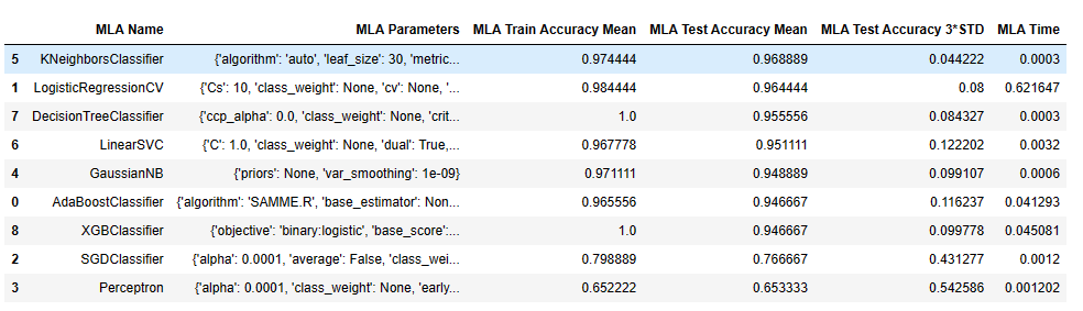
使用多个模型测试
#create table to compare MLA predictions
# train['pred']=-1
MLA_predict={}
MLA_predict['true'] = iris.target

#index through MLA and save performance to table
row_index = 0
for alg in MLA:

    #set name and parameters
    MLA_name = alg.__class__.__name__
    print(MLA_name)
    MLA_compare.loc[row_index, 'MLA Name'] = MLA_name
    MLA_compare.loc[row_index, 'MLA Parameters'] = str(alg.get_params())
    cv_results = model_selection.cross_validate(alg,
                 iris.data,iris.target, cv  = cv_split,return_train_score=True)

    MLA_compare.loc[row_index, 'MLA Time'] = cv_results['fit_time'].mean()
    MLA_compare.loc[row_index, 'MLA Train Accuracy Mean'] = cv_results['train_score'].mean()
    MLA_compare.loc[row_index, 'MLA Test Accuracy Mean'] = cv_results['test_score'].mean()
    #if this is a non-bias random sample, then +/-3 standard deviations (std) from the mean, should statistically capture 99.7% of the subsets
    MLA_compare.loc[row_index, 'MLA Test Accuracy 3*STD'] = cv_results['test_score'].std()*3   #let's know the worst that can happen!


    #save MLA predictions - see section 6 for usage
    alg.fit(iris.data, iris.target)
    MLA_predict[MLA_name] = alg.predict(iris.data)

    row_index+=1

MLA_compare.sort_values(by = ['MLA Test Accuracy Mean'], ascending = False, inplace = True)
MLA_compare
输出为:
AdaBoostClassifier
LogisticRegressionCV
SGDClassifier
Perceptron
GaussianNB
KNeighborsClassifier
LinearSVC
DecisionTreeClassifier
XGBClassifier
MLA_predict
输出为:
{‘true’: array([0, 0, 0, 0, 0, 0, 0, 0, 0, 0, 0, 0, 0, 0, 0, 0, 0, 0, 0, 0, 0, 0,
0, 0, 0, 0, 0, 0, 0, 0, 0, 0, 0, 0, 0, 0, 0, 0, 0, 0, 0, 0, 0, 0,
0, 0, 0, 0, 0, 0, 1, 1, 1, 1, 1, 1, 1, 1, 1, 1, 1, 1, 1, 1, 1, 1,
1, 1, 1, 1, 1, 1, 1, 1, 1, 1, 1, 1, 1, 1, 1, 1, 1, 1, 1, 1, 1, 1,
1, 1, 1, 1, 1, 1, 1, 1, 1, 1, 1, 1, 2, 2, 2, 2, 2, 2, 2, 2, 2, 2,
2, 2, 2, 2, 2, 2, 2, 2, 2, 2, 2, 2, 2, 2, 2, 2, 2, 2, 2, 2, 2, 2,
2, 2, 2, 2, 2, 2, 2, 2, 2, 2, 2, 2, 2, 2, 2, 2, 2, 2]),
‘AdaBoostClassifier’: array([0, 0, 0, 0, 0, 0, 0, 0, 0, 0, 0, 0, 0, 0, 0, 0, 0, 0, 0, 0, 0, 0,
0, 0, 0, 0, 0, 0, 0, 0, 0, 0, 0, 0, 0, 0, 0, 0, 0, 0, 0, 0, 0, 0,
0, 0, 0, 0, 0, 0, 1, 1, 1, 1, 1, 1, 1, 1, 1, 1, 1, 1, 1, 1, 1, 1,
1, 1, 1, 1, 2, 1, 1, 1, 1, 1, 1, 2, 1, 1, 1, 1, 1, 1, 1, 1, 1, 1,
1, 1, 1, 1, 1, 1, 1, 1, 1, 1, 1, 1, 2, 2, 2, 2, 2, 2, 2, 2, 2, 2,
2, 2, 2, 2, 2, 2, 2, 2, 2, 1, 2, 2, 2, 2, 2, 2, 2, 2, 2, 1, 2, 2,
2, 1, 1, 2, 2, 2, 2, 2, 2, 2, 2, 2, 2, 2, 2, 2, 2, 2]),
‘LogisticRegressionCV’: array([0, 0, 0, 0, 0, 0, 0, 0, 0, 0, 0, 0, 0, 0, 0, 0, 0, 0, 0, 0, 0, 0,
0, 0, 0, 0, 0, 0, 0, 0, 0, 0, 0, 0, 0, 0, 0, 0, 0, 0, 0, 0, 0, 0,
0, 0, 0, 0, 0, 0, 1, 1, 1, 1, 1, 1, 1, 1, 1, 1, 1, 1, 1, 1, 1, 1,
1, 1, 1, 1, 2, 1, 1, 1, 1, 1, 1, 1, 1, 1, 1, 1, 1, 2, 1, 1, 1, 1,
1, 1, 1, 1, 1, 1, 1, 1, 1, 1, 1, 1, 2, 2, 2, 2, 2, 2, 2, 2, 2, 2,
2, 2, 2, 2, 2, 2, 2, 2, 2, 2, 2, 2, 2, 2, 2, 2, 2, 2, 2, 2, 2, 2,
2, 1, 2, 2, 2, 2, 2, 2, 2, 2, 2, 2, 2, 2, 2, 2, 2, 2]),
‘SGDClassifier’: array([0, 0, 0, 0, 0, 0, 0, 0, 0, 0, 0, 0, 0, 0, 0, 0, 0, 0, 0, 0, 0, 0,
0, 0, 0, 0, 0, 0, 0, 0, 0, 0, 0, 0, 0, 0, 0, 0, 0, 0, 0, 0, 0, 0,
0, 0, 0, 0, 0, 0, 0, 0, 0, 1, 2, 2, 2, 0, 0, 2, 1, 0, 1, 2, 0, 0,
2, 1, 2, 1, 2, 0, 2, 2, 0, 0, 1, 2, 2, 0, 1, 1, 0, 2, 2, 2, 0, 1,
0, 0, 2, 2, 0, 0, 2, 0, 0, 0, 0, 0, 2, 2, 2, 2, 2, 2, 2, 2, 2, 2,
2, 2, 2, 2, 2, 2, 2, 2, 2, 2, 2, 2, 2, 2, 2, 2, 2, 2, 2, 2, 2, 2,
2, 2, 2, 2, 2, 2, 2, 2, 2, 2, 2, 2, 2, 2, 2, 2, 2, 2]),
‘Perceptron’: array([1, 1, 1, 1, 1, 1, 0, 1, 1, 1, 1, 1, 1, 1, 0, 0, 0, 1, 1, 0, 1, 0,
0, 1, 1, 1, 1, 1, 1, 1, 1, 1, 0, 0, 1, 1, 1, 1, 1, 1, 1, 1, 1, 1,
1, 1, 1, 1, 1, 1, 1, 1, 1, 1, 1, 1, 1, 1, 1, 1, 1, 1, 1, 1, 1, 1,
1, 1, 1, 1, 1, 1, 1, 1, 1, 1, 1, 1, 1, 1, 1, 1, 1, 1, 1, 1, 1, 1,
1, 1, 1, 1, 1, 1, 1, 1, 1, 1, 1, 1, 2, 1, 1, 1, 2, 1, 2, 1, 1, 2,
1, 1, 1, 2, 2, 1, 1, 1, 1, 1, 1, 2, 1, 1, 1, 1, 1, 1, 1, 1, 1, 1,
2, 1, 1, 1, 2, 1, 1, 1, 2, 1, 1, 2, 2, 1, 1, 1, 2, 1]),
‘GaussianNB’: array([0, 0, 0, 0, 0, 0, 0, 0, 0, 0, 0, 0, 0, 0, 0, 0, 0, 0, 0, 0, 0, 0,
0, 0, 0, 0, 0, 0, 0, 0, 0, 0, 0, 0, 0, 0, 0, 0, 0, 0, 0, 0, 0, 0,
0, 0, 0, 0, 0, 0, 1, 1, 2, 1, 1, 1, 1, 1, 1, 1, 1, 1, 1, 1, 1, 1,
1, 1, 1, 1, 2, 1, 1, 1, 1, 1, 1, 2, 1, 1, 1, 1, 1, 1, 1, 1, 1, 1,
1, 1, 1, 1, 1, 1, 1, 1, 1, 1, 1, 1, 2, 2, 2, 2, 2, 2, 1, 2, 2, 2,
2, 2, 2, 2, 2, 2, 2, 2, 2, 1, 2, 2, 2, 2, 2, 2, 2, 2, 2, 2, 2, 2,
2, 1, 2, 2, 2, 2, 2, 2, 2, 2, 2, 2, 2, 2, 2, 2, 2, 2]),
‘KNeighborsClassifier’: array([0, 0, 0, 0, 0, 0, 0, 0, 0, 0, 0, 0, 0, 0, 0, 0, 0, 0, 0, 0, 0, 0,
0, 0, 0, 0, 0, 0, 0, 0, 0, 0, 0, 0, 0, 0, 0, 0, 0, 0, 0, 0, 0, 0,
0, 0, 0, 0, 0, 0, 1, 1, 1, 1, 1, 1, 1, 1, 1, 1, 1, 1, 1, 1, 1, 1,
1, 1, 1, 1, 2, 1, 2, 1, 1, 1, 1, 1, 1, 1, 1, 1, 1, 2, 1, 1, 1, 1,
1, 1, 1, 1, 1, 1, 1, 1, 1, 1, 1, 1, 2, 2, 2, 2, 2, 2, 1, 2, 2, 2,
2, 2, 2, 2, 2, 2, 2, 2, 2, 1, 2, 2, 2, 2, 2, 2, 2, 2, 2, 2, 2, 2,
2, 2, 2, 2, 2, 2, 2, 2, 2, 2, 2, 2, 2, 2, 2, 2, 2, 2]),
‘LinearSVC’: array([0, 0, 0, 0, 0, 0, 0, 0, 0, 0, 0, 0, 0, 0, 0, 0, 0, 0, 0, 0, 0, 0,
0, 0, 0, 0, 0, 0, 0, 0, 0, 0, 0, 0, 0, 0, 0, 0, 0, 0, 0, 0, 0, 0,
0, 0, 0, 0, 0, 0, 1, 1, 1, 1, 1, 1, 1, 1, 1, 1, 1, 1, 1, 1, 1, 1,
1, 1, 1, 1, 2, 1, 1, 1, 1, 1, 1, 1, 1, 1, 1, 1, 1, 2, 2, 1, 1, 1,
1, 1, 1, 1, 1, 1, 1, 1, 1, 1, 1, 1, 2, 2, 2, 2, 2, 2, 2, 2, 2, 2,
2, 2, 2, 2, 2, 2, 2, 2, 2, 2, 2, 2, 2, 2, 2, 2, 2, 2, 2, 1, 2, 2,
2, 1, 2, 2, 2, 2, 2, 2, 2, 2, 2, 2, 2, 2, 2, 2, 2, 2]),
‘DecisionTreeClassifier’: array([0, 0, 0, 0, 0, 0, 0, 0, 0, 0, 0, 0, 0, 0, 0, 0, 0, 0, 0, 0, 0, 0,
0, 0, 0, 0, 0, 0, 0, 0, 0, 0, 0, 0, 0, 0, 0, 0, 0, 0, 0, 0, 0, 0,
0, 0, 0, 0, 0, 0, 1, 1, 1, 1, 1, 1, 1, 1, 1, 1, 1, 1, 1, 1, 1, 1,
1, 1, 1, 1, 1, 1, 1, 1, 1, 1, 1, 1, 1, 1, 1, 1, 1, 1, 1, 1, 1, 1,
1, 1, 1, 1, 1, 1, 1, 1, 1, 1, 1, 1, 2, 2, 2, 2, 2, 2, 2, 2, 2, 2,
2, 2, 2, 2, 2, 2, 2, 2, 2, 2, 2, 2, 2, 2, 2, 2, 2, 2, 2, 2, 2, 2,
2, 2, 2, 2, 2, 2, 2, 2, 2, 2, 2, 2, 2, 2, 2, 2, 2, 2]),
‘XGBClassifier’: array([0, 0, 0, 0, 0, 0, 0, 0, 0, 0, 0, 0, 0, 0, 0, 0, 0, 0, 0, 0, 0, 0,
0, 0, 0, 0, 0, 0, 0, 0, 0, 0, 0, 0, 0, 0, 0, 0, 0, 0, 0, 0, 0, 0,
0, 0, 0, 0, 0, 0, 1, 1, 1, 1, 1, 1, 1, 1, 1, 1, 1, 1, 1, 1, 1, 1,
1, 1, 1, 1, 1, 1, 1, 1, 1, 1, 1, 1, 1, 1, 1, 1, 1, 1, 1, 1, 1, 1,
1, 1, 1, 1, 1, 1, 1, 1, 1, 1, 1, 1, 2, 2, 2, 2, 2, 2, 2, 2, 2, 2,
2, 2, 2, 2, 2, 2, 2, 2, 2, 2, 2, 2, 2, 2, 2, 2, 2, 2, 2, 2, 2, 2,
2, 2, 2, 2, 2, 2, 2, 2, 2, 2, 2, 2, 2, 2, 2, 2, 2, 2], dtype=int64)}
cv_results
输出为:
{‘fit_time’: array([1.16533065, 0.02996469, 0.03700185, 0.03500032, 0.02999783,
0.03499651, 0.03400135, 0.03099895, 0.03699994, 0.0380013 ]),
‘score_time’: array([0. , 0. , 0.00099874, 0.00100255, 0. ,
0. , 0.00099492, 0. , 0.00100017, 0.00099897]),
‘test_score’: array([0.97777778, 0.91111111, 0.95555556, 0.93333333, 0.97777778,
0.91111111, 0.97777778, 1. , 0.97777778, 0.97777778]),
‘train_score’: array([1., 1., 1., 1., 1., 1., 1., 1., 1., 1.])}
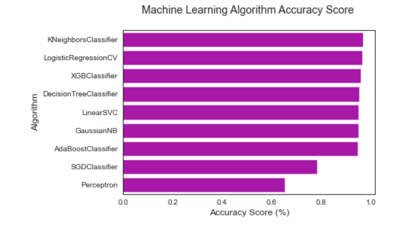
进行绘图:
#柱状图  https://seaborn.pydata.org/generated/seaborn.barplot.html
sns.barplot(x='MLA Test Accuracy Mean', y = 'MLA Name', data = MLA_compare, color = 'm')

#pyplot 美化: https://matplotlib.org/api/pyplot_api.html
plt.title('Machine Learning Algorithm Accuracy Score \n')
plt.xlabel('Accuracy Score (%)')
plt.ylabel('Algorithm')
输出为:
多个模型投票
vote_est = [
#Ensemble Methods: http://scikit-learn.org/stable/modules/ensemble.html
('ada', ensemble.AdaBoostClassifier()),
# ('bc', ensemble.BaggingClassifier()),
# ('etc',ensemble.ExtraTreesClassifier()),
# ('gbc', ensemble.GradientBoostingClassifier()),
# ('rfc', ensemble.RandomForestClassifier()),
#Gaussian Processes: http://scikit-learn.org/stable/modules/gaussian_process.html#gaussian-process-classification-gpc
# ('gpc', gaussian_process.GaussianProcessClassifier()),
#GLM: http://scikit-learn.org/stable/modules/linear_model.html#logistic-regression
('lr', linear_model.LogisticRegressionCV()),
#Navies Bayes: http://scikit-learn.org/stable/modules/naive_bayes.html
# ('bnb', naive_bayes.BernoulliNB()),
('gnb', naive_bayes.GaussianNB()),
#Nearest Neighbor: http://scikit-learn.org/stable/modules/neighbors.html
('knn', neighbors.KNeighborsClassifier()),
#SVM: http://scikit-learn.org/stable/modules/svm.html
('svc', svm.SVC(probability=True)),
('xgb', XGBClassifier())
]
# iris.data,iris.target
#多数投票
vote_hard = ensemble.VotingClassifier(estimators = vote_est , voting = 'hard')
vote_hard_cv = model_selection.cross_validate(vote_hard, iris.data,iris.target, cv = cv_split,return_train_score=True)
vote_hard.fit(iris.data,iris.target)
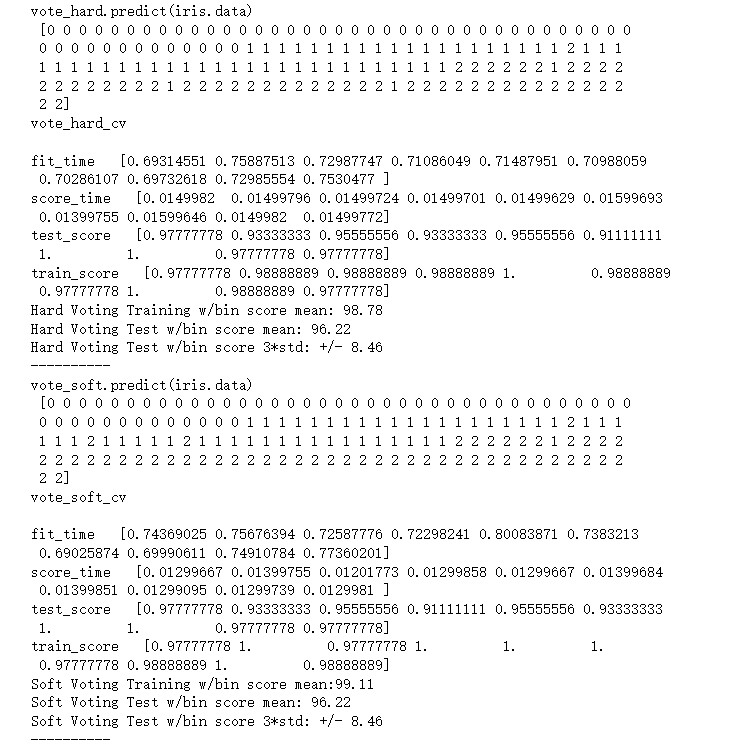
print("vote_hard.predict(iris.data)\n",vote_hard.predict(iris.data))
print("vote_hard_cv\n")
for k,v in vote_hard_cv.items():
print(k," ",v)
print("Hard Voting Training w/bin score mean: {:.2f}". format(vote_hard_cv['train_score'].mean()*100))
print("Hard Voting Test w/bin score mean: {:.2f}". format(vote_hard_cv['test_score'].mean()*100))
print("Hard Voting Test w/bin score 3*std: +/- {:.2f}". format(vote_hard_cv['test_score'].std()*100*3))
print('-'*10)
#权重投票
vote_soft = ensemble.VotingClassifier(estimators = vote_est , voting = 'soft')
vote_soft_cv = model_selection.cross_validate(vote_soft, iris.data,iris.target, cv = cv_split,return_train_score=True)
vote_soft.fit(iris.data,iris.target)
print("vote_soft.predict(iris.data)\n",vote_soft.predict(iris.data))
print("vote_soft_cv\n")
for k,v in vote_soft_cv.items():
print(k," ",v)
print("Soft Voting Training w/bin score mean:{:.2f}". format(vote_soft_cv['train_score'].mean()*100))
print("Soft Voting Test w/bin score mean: {:.2f}". format(vote_soft_cv['test_score'].mean()*100))
print("Soft Voting Test w/bin score 3*std: +/- {:.2f}". format(vote_soft_cv['test_score'].std()*100*3))
print('-'*10)
输出为:
完整代码
import sys
import os
print("Python version: {}". format(sys.version))
import pandas as pd # 加载csv等表格数据
print("pandas version: {}". format(pd.__version__))

import matplotlib # 画图
print("matplotlib version: {}". format(matplotlib.__version__))

import numpy as np #数据运算
print("NumPy version: {}". format(np.__version__))

import scipy as sp #高级数学运算
print("SciPy version: {}". format(sp.__version__))

import IPython
from IPython import display #美化DataFrame的输出


import sklearn #机器学习算法
print("scikit-learn version: {}". format(sklearn.__version__))

#基础库
import random
import time


#忽略警告
import warnings
warnings.filterwarnings('ignore')
print('-'*25)


# 常见机器学习算法
from sklearn import svm, tree, linear_model, neighbors, naive_bayes, ensemble, discriminant_analysis, gaussian_process
from xgboost import XGBClassifier

from sklearn import datasets

# 常见函数
from sklearn.preprocessing import OneHotEncoder, LabelEncoder
from sklearn import feature_selection
from sklearn import model_selection
from sklearn import metrics

#可视化
import matplotlib as mpl
import matplotlib.pyplot as plt
import matplotlib.pylab as pylab
import seaborn as sns
from pandas.plotting import scatter_matrix


#配置可视化
%matplotlib inline
mpl.style.use('ggplot')
sns.set_style('white')
pylab.rcParams['figure.figsize'] = 12,8

MLA = [
    #集成方法
    ensemble.AdaBoostClassifier(),
    # ensemble.BaggingClassifier(),
    # ensemble.ExtraTreesClassifier(),
    # ensemble.GradientBoostingClassifier(),
    # ensemble.RandomForestClassifier(),

    #高斯过程
    # gaussian_process.GaussianProcessClassifier(),

    #非线性分类器
    linear_model.LogisticRegressionCV(),
    # linear_model.PassiveAggressiveClassifier(),
    # linear_model.RidgeClassifierCV(),
    linear_model.SGDClassifier(),
    linear_model.Perceptron(),

    #贝叶斯
    # naive_bayes.BernoulliNB(),
    naive_bayes.GaussianNB(),

    #KNN算法
    neighbors.KNeighborsClassifier(),

    #支持向量机-SVM
    # svm.SVC(probability=True),
    # svm.NuSVC(probability=True),
    svm.LinearSVC(),

    #决策树模型
    tree.DecisionTreeClassifier(),
    # tree.ExtraTreeClassifier(),

    #奇异值分析
    # discriminant_analysis.LinearDiscriminantAnalysis(),
    # discriminant_analysis.QuadraticDiscriminantAnalysis(),


    #xgboost: http://xgboost.readthedocs.io/en/latest/model.html
    XGBClassifier()
    ]

iris = datasets.load_iris()
iris.data
iris.target
# X_train, X_test, y_train, y_test = train_test_split(
#     iris.data, iris.target, test_size=0.4, random_state=0)
cv_split = model_selection.ShuffleSplit(n_splits = 10, test_size = .3, train_size = .6, random_state = 0 ) # run model 10x with 60/30 split intentionally leaving out 10%

#create table to compare MLA metrics
MLA_columns = ['MLA Name', 'MLA Parameters','MLA Train Accuracy Mean', 'MLA Test Accuracy Mean', 'MLA Test Accuracy 3*STD' ,'MLA Time']
MLA_compare = pd.DataFrame(columns = MLA_columns)
MLA_compare

#create table to compare MLA predictions
# train['pred']=-1
MLA_predict={}
MLA_predict['true'] = iris.target

#index through MLA and save performance to table
row_index = 0
for alg in MLA:

    #set name and parameters
    MLA_name = alg.__class__.__name__
    print(MLA_name)
    MLA_compare.loc[row_index, 'MLA Name'] = MLA_name
    MLA_compare.loc[row_index, 'MLA Parameters'] = str(alg.get_params())
    cv_results = model_selection.cross_validate(alg,
                 iris.data,iris.target, cv  = cv_split,return_train_score=True)

    MLA_compare.loc[row_index, 'MLA Time'] = cv_results['fit_time'].mean()
    MLA_compare.loc[row_index, 'MLA Train Accuracy Mean'] = cv_results['train_score'].mean()
    MLA_compare.loc[row_index, 'MLA Test Accuracy Mean'] = cv_results['test_score'].mean()
    #if this is a non-bias random sample, then +/-3 standard deviations (std) from the mean, should statistically capture 99.7% of the subsets
    MLA_compare.loc[row_index, 'MLA Test Accuracy 3*STD'] = cv_results['test_score'].std()*3   #let's know the worst that can happen!


    #save MLA predictions - see section 6 for usage
    alg.fit(iris.data, iris.target)
    MLA_predict[MLA_name] = alg.predict(iris.data)

    row_index+=1

MLA_compare.sort_values(by = ['MLA Test Accuracy Mean'], ascending = False, inplace = True)
MLA_compare

MLA_predict

cv_results

#柱状图  https://seaborn.pydata.org/generated/seaborn.barplot.html
sns.barplot(x='MLA Test Accuracy Mean', y = 'MLA Name', data = MLA_compare, color = 'm')

#pyplot 美化: https://matplotlib.org/api/pyplot_api.html
plt.title('Machine Learning Algorithm Accuracy Score \n')
plt.xlabel('Accuracy Score (%)')
plt.ylabel('Algorithm')


vote_est = [
    #Ensemble Methods: http://scikit-learn.org/stable/modules/ensemble.html
    ('ada', ensemble.AdaBoostClassifier()),
    # ('bc', ensemble.BaggingClassifier()),
    # ('etc',ensemble.ExtraTreesClassifier()),
    # ('gbc', ensemble.GradientBoostingClassifier()),
    # ('rfc', ensemble.RandomForestClassifier()),

    #Gaussian Processes: http://scikit-learn.org/stable/modules/gaussian_process.html#gaussian-process-classification-gpc
    # ('gpc', gaussian_process.GaussianProcessClassifier()),

    #GLM: http://scikit-learn.org/stable/modules/linear_model.html#logistic-regression
    ('lr', linear_model.LogisticRegressionCV()),

    #Navies Bayes: http://scikit-learn.org/stable/modules/naive_bayes.html
    # ('bnb', naive_bayes.BernoulliNB()),
    ('gnb', naive_bayes.GaussianNB()),

    #Nearest Neighbor: http://scikit-learn.org/stable/modules/neighbors.html
    ('knn', neighbors.KNeighborsClassifier()),

    #SVM: http://scikit-learn.org/stable/modules/svm.html
    ('svc', svm.SVC(probability=True)),
    ('xgb', XGBClassifier())

]

# iris.data,iris.target
#多数投票
vote_hard = ensemble.VotingClassifier(estimators = vote_est , voting = 'hard')
vote_hard_cv = model_selection.cross_validate(vote_hard, iris.data,iris.target, cv  = cv_split,return_train_score=True)
vote_hard.fit(iris.data,iris.target)

print("vote_hard.predict(iris.data)\n",vote_hard.predict(iris.data))

print("vote_hard_cv\n")
for k,v in vote_hard_cv.items():
    print(k," ",v)

print("Hard Voting Training w/bin score mean: {:.2f}". format(vote_hard_cv['train_score'].mean()*100))
print("Hard Voting Test w/bin score mean: {:.2f}". format(vote_hard_cv['test_score'].mean()*100))
print("Hard Voting Test w/bin score 3*std: +/- {:.2f}". format(vote_hard_cv['test_score'].std()*100*3))
print('-'*10)


#权重投票
vote_soft = ensemble.VotingClassifier(estimators = vote_est , voting = 'soft')
vote_soft_cv = model_selection.cross_validate(vote_soft, iris.data,iris.target, cv  = cv_split,return_train_score=True)
vote_soft.fit(iris.data,iris.target)
print("vote_soft.predict(iris.data)\n",vote_soft.predict(iris.data))
print("vote_soft_cv\n")
for k,v in vote_soft_cv.items():
    print(k," ",v)


print("Soft Voting Training w/bin score mean:{:.2f}". format(vote_soft_cv['train_score'].mean()*100))
print("Soft Voting Test w/bin score mean: {:.2f}". format(vote_soft_cv['test_score'].mean()*100))
print("Soft Voting Test w/bin score 3*std: +/- {:.2f}". format(vote_soft_cv['test_score'].std()*100*3))
print('-'*10)