机器学习之分类回归模型（决策数、随机森林）

回归分析

回归分析属于监督学习方法的一种，主要用于预测连续型目标变量，可以预测、计算趋势以及确定变量之间的关系等。

Regession Evaluation Metrics

以下是一些最流行的回归评估指标:
平均绝对误差(MAE):目标变量的预测值与实际值之间的平均绝对差值。
均方误差(MSE):目标变量的预测值与实际值之间的平均平方差。
均方根误差(RMSE):均方根误差的平方根。
Huber Loss:一种混合损失函数，在较大误差时从MAE过渡到MSE，在鲁棒性和MSE对异常值的敏感性之间提供平衡。
均方根对数误差
R2-Score

分类模型

决策树(监督分类回归模型)

分类树:该树用于确定目标变量在连续时最有可能落入哪个“类”。
回归树:用于预测连续变量的值。
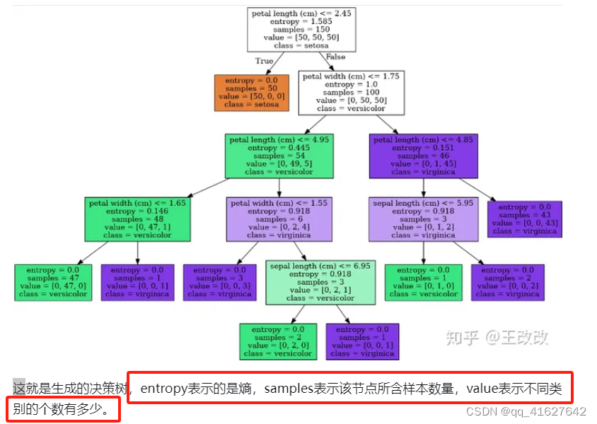
在决策树中，节点根据属性的阈值划分为子节点。将根节点作为训练集，并根据最优属性和阈值将其分割为两个节点。此外，子集也使用相同的逻辑进行分割。这个过程一直持续，直到在树中找到最后一个纯子集，或者在该生长的树中找到最大可能的叶子数。
在这里插入图片描述

根据分割指标和分割方法，可分为：ID3、C4.5、CART算法。
（1）ID3算法：以信息增益为准则来选择最优划分属性
信息增益的计算是基于信息熵（度量样本集合纯度的指标）
在这里插入图片描述

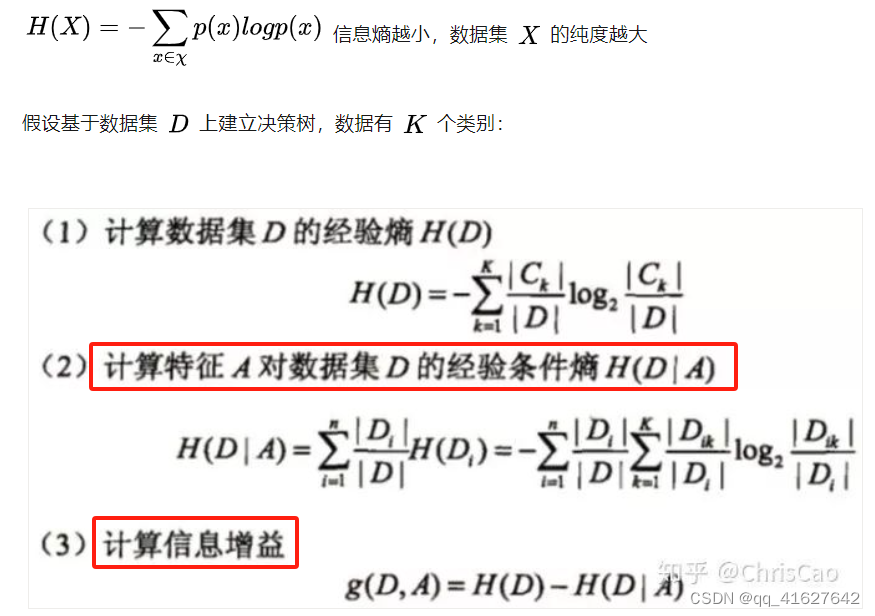
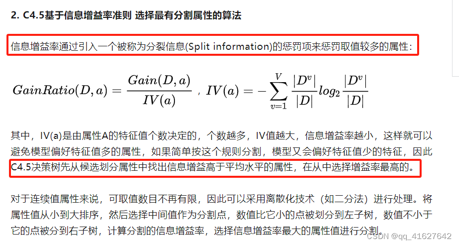
（2）C4.5基于信息增益率准则选择最有分割属性的算法

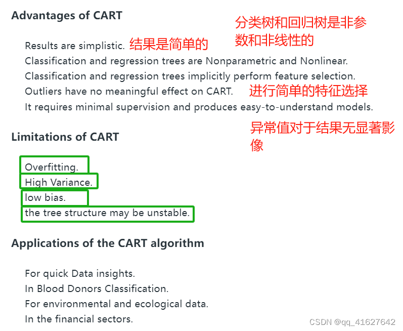
3. CART:以基尼系数为准则选择最优划分属性，可用于分类和回归
基尼杂质-基尼杂质测量根据多数类标记的子集对随机实例进行错误分类的概率。基尼不纯系数越低，意味着子集的纯度越高。分割标准- CART算法评估每个节点上的所有潜在分割，并选择最能减少结果子集的基尼杂质的分割。这个过程一直持续，直到达到一个停止条件，比如最大树深度或叶子节点中的最小实例数。

在这里插入图片描述

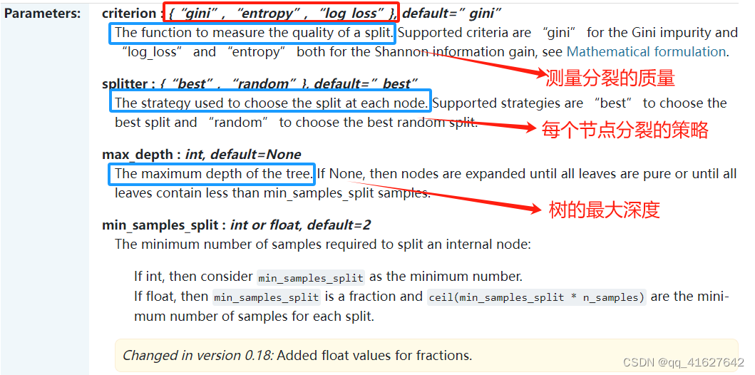
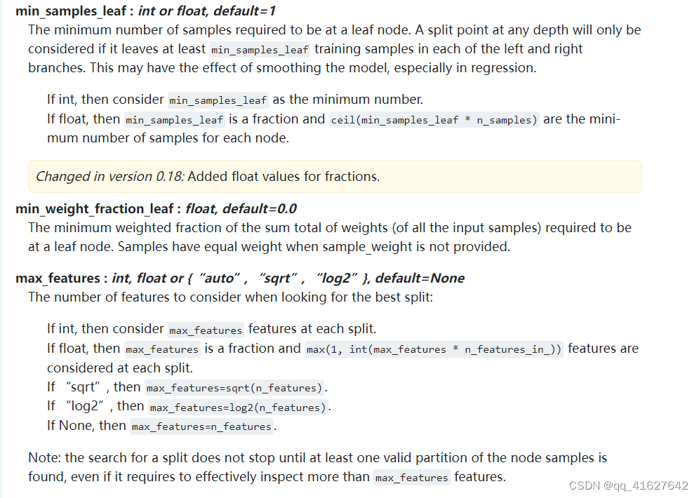
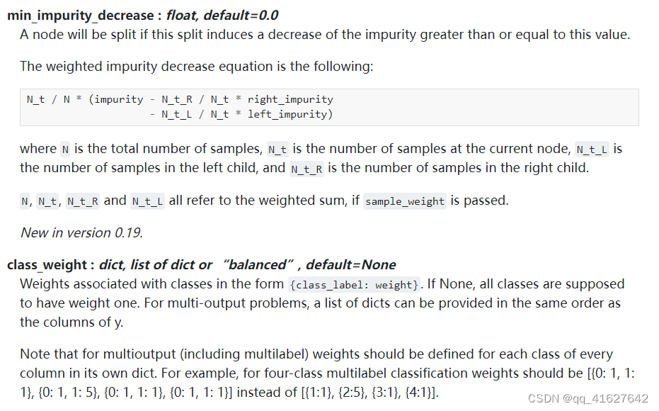
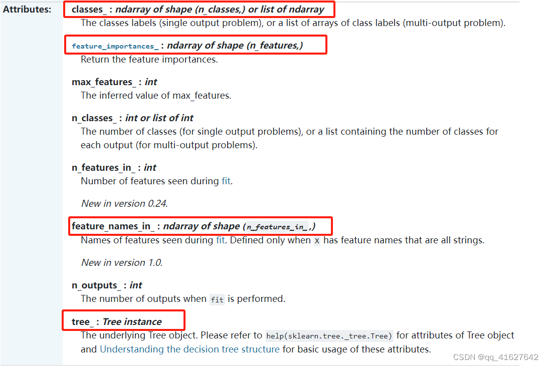
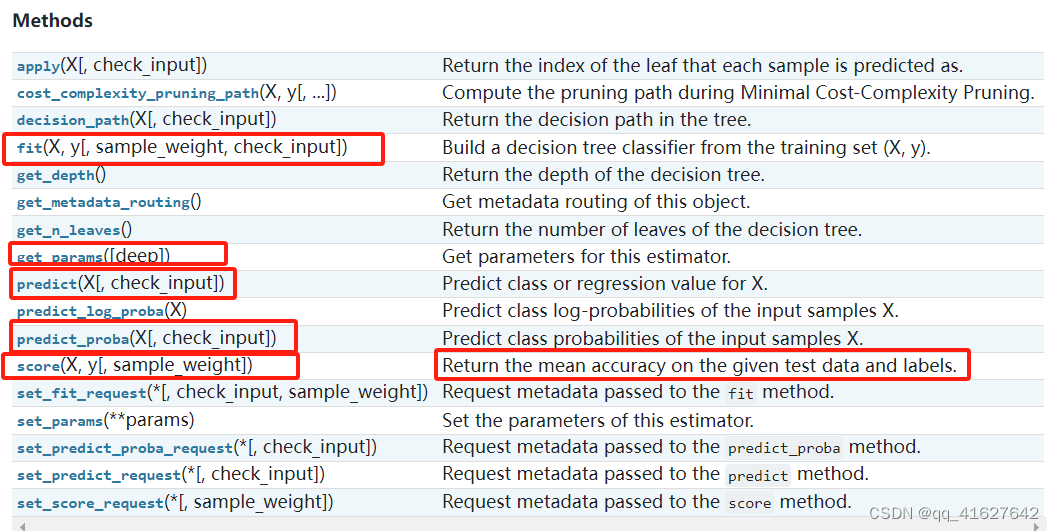
sklearn.tree.DecisionTreeClassifier（分类）

class sklearn.tree.DecisionTreeClassifier(*, criterion='gini', splitter='best', max_depth=None, min_samples_split=2, min_samples_leaf=1, min_weight_fraction_leaf=0.0, max_features=None, random_state=None, max_leaf_nodes=None, min_impurity_decrease=0.0, class_weight=None, ccp_alpha=0.0)[source]

在这里插入图片描述

from sklearn.tree import DecisionTreeClassifier
from sklearn.model_selection import train_test_split
cancer = load_breast_cancer()
X_train, X_test, y_train, y_test = train_test_split(
    cancer.data, cancer.target, stratify=cancer.target, random_state=42)
tree = DecisionTreeClassifier(random_state=0)
tree.fit(X_train, y_train)
print("Accuracy on training set: {:.3f}".format(tree.score(X_train, y_train)))
print("Accuracy on test set: {:.3f}".format(tree.score(X_test, y_test)))

tree = DecisionTreeClassifier(max_depth=4, random_state=0)
tree.fit(X_train, y_train)

print("Accuracy on training set: {:.3f}".format(tree.score(X_train, y_train)))
print("Accuracy on test set: {:.3f}".format(tree.score(X_test, y_test)))

fig, axes = plt.subplots(2, 3, figsize=(20, 10))
for i, (ax, tree) in enumerate(zip(axes.ravel(), forest.estimators_)):
    ax.set_title("Tree {}".format(i))
    mglearn.plots.plot_tree_partition(X_train, y_train, tree, ax=ax)
    
mglearn.plots.plot_2d_separator(forest, X_train, fill=True, ax=axes[-1, -1],
                                alpha=.4)
axes[-1, -1].set_title("Random Forest")
mglearn.discrete_scatter(X_train[:, 0], X_train[:, 1], y_train)

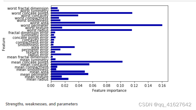
def plot_feature_importances_cancer(model):
    n_features = cancer.data.shape[1]
    plt.barh(np.arange(n_features), model.feature_importances_, align='center')
    plt.yticks(np.arange(n_features), cancer.feature_names)
    plt.xlabel("Feature importance")
    plt.ylabel("Feature")
    plt.ylim(-1, n_features)

plot_feature_importances_cancer(tree)

在这里插入图片描述

from sklearn.tree import DecisionTreeClassifier
from sklearn.preprocessing import LabelEncoder
 
# Define the features and target variable
features = [
    ["red", "large"],
    ["green", "small"],
    ["red", "small"],
    ["yellow", "large"],
    ["green", "large"],
    ["orange", "large"],
]
target_variable = ["apple", "lime", "strawberry", "banana", "grape", "orange"]
 
# Flatten the features list for encoding
flattened_features = [item for sublist in features for item in sublist]
 
# Use a single LabelEncoder for all features and target variable
le = LabelEncoder()
le.fit(flattened_features + target_variable)
 
# Encode features and target variable
encoded_features = [le.transform(item) for item in features]
encoded_target = le.transform(target_variable)
 
# Create a CART classifier
clf = DecisionTreeClassifier()
 
# Train the classifier on the training set
clf.fit(encoded_features, encoded_target)
 
# Predict the fruit type for a new instance
new_instance = ["red", "large"]
encoded_new_instance = le.transform(new_instance)
predicted_fruit_type = clf.predict([encoded_new_instance])
decoded_predicted_fruit_type = le.inverse_transform(predicted_fruit_type)
print("Predicted fruit type:", decoded_predicted_fruit_type[0])

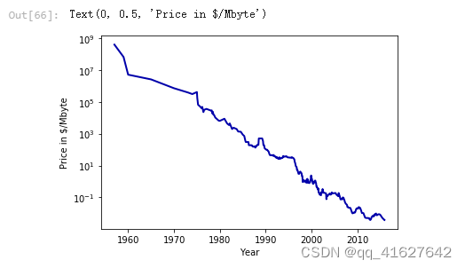
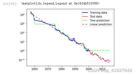
DecisionTreeRegressor（回归）

import os
ram_prices = pd.read_csv(os.path.join(mglearn.datasets.DATA_PATH, "ram_price.csv"))

plt.semilogy(ram_prices.date, ram_prices.price)
plt.xlabel("Year")
plt.ylabel("Price in $/Mbyte")

在这里插入图片描述

from sklearn.tree import DecisionTreeRegressor
# use historical data to forecast prices after the year 2000
data_train = ram_prices[ram_prices.date < 2000]
data_test = ram_prices[ram_prices.date >= 2000]

# predict prices based on date
X_train = data_train.date[:, np.newaxis]
# we use a log-transform to get a simpler relationship of data to target
y_train = np.log(data_train.price)

tree = DecisionTreeRegressor(max_depth=3).fit(X_train, y_train)
linear_reg = LinearRegression().fit(X_train, y_train)

# predict on all data
X_all = ram_prices.date[:, np.newaxis]

pred_tree = tree.predict(X_all)
pred_lr = linear_reg.predict(X_all)

# undo log-transform
price_tree = np.exp(pred_tree)
price_lr = np.exp(pred_lr)

plt.semilogy(data_train.date, data_train.price, label="Training data")
plt.semilogy(data_test.date, data_test.price, label="Test data")
plt.semilogy(ram_prices.date, price_tree, label="Tree prediction")
plt.semilogy(ram_prices.date, price_lr, label="Linear prediction")
plt.legend()

在这里插入图片描述

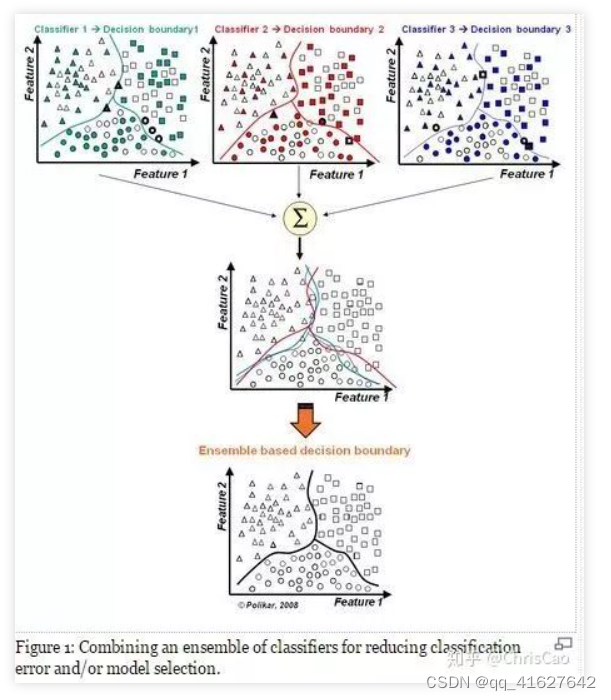
随机森林（集成学习）

先补充组合分类器的概念，将多个分类器的结果进行多票表决或取平均值，以此作为最终的结果。
每个决策树都有很高的方差，但是当我们将它们并行地组合在一起时，结果的方差就会很低，因为每个决策树都在特定的样本数据上得到了完美的训练，因此输出不依赖于一个决策树，而是依赖于多个决策树。在分类问题的情况下，使用多数投票分类器获得最终输出。在回归问题的情况下，最终输出是所有输出的平均值。这部分称为聚合。
1.构建组合分类器的好处：
(1)提升模型精度：整合各个模型的分类结果，得到更合理的决策边界，减少整体错误呢，实现更好的分类效果：
在这里插入图片描述
(2)处理过大或过小的数据集：数据集较大时，可将数据集划分成多个子集，对子集构建分类器；当数据集较小时，通过自助采样(bootstrap)从原始数据集采样产生多组不同的数据集，构建分类器。

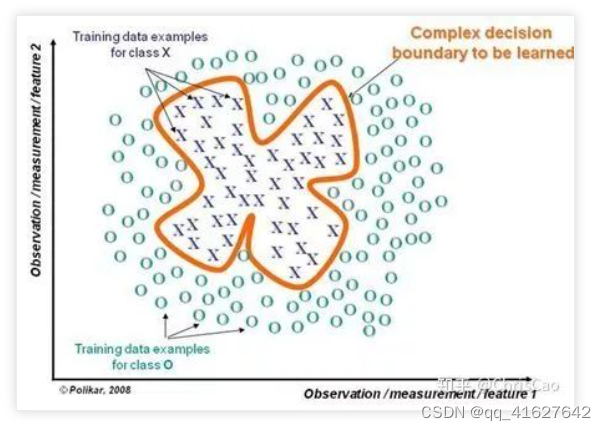
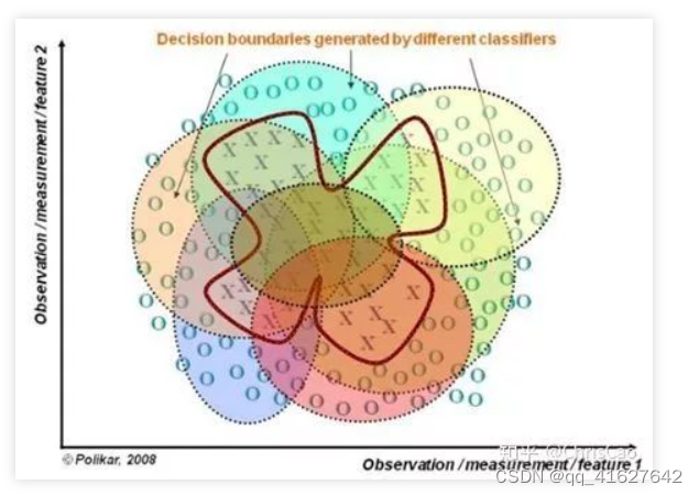
(3)若决策边界过于复杂，则线性模型不能很好地描述真实情况。因此，现对于特定区域的数据集，训练多个线性分类器，再将他们集成。
在这里插入图片描述
(4)比较适合处理多源异构数据（存储方式不同（关系型、非关系型），类别不同（时序型、离散型、连续型、网络结构数据））

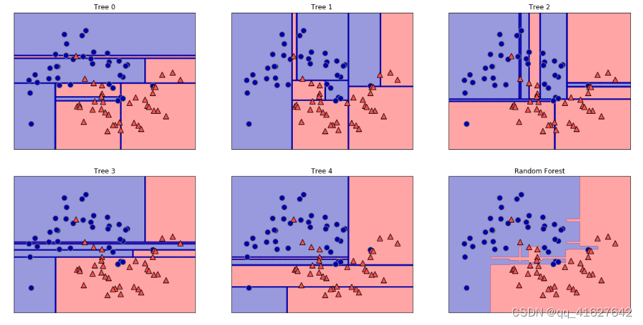
随机森林是一个多决策树的组合分类器，随机主要体现在两个方面：数据选取的随机性和特征选取的随机性。
在这里插入图片描述

from sklearn.ensemble import RandomForestClassifier
from sklearn.datasets import make_moons

X, y = make_moons(n_samples=100, noise=0.25, random_state=3)
X_train, X_test, y_train, y_test = train_test_split(X, y, stratify=y,
                                                    random_state=42)

forest = RandomForestClassifier(n_estimators=5, random_state=2)
forest.fit(X_train, y_train)

fig, axes = plt.subplots(2, 3, figsize=(20, 10))
for i, (ax, tree) in enumerate(zip(axes.ravel(), forest.estimators_)):
    ax.set_title("Tree {}".format(i))
    mglearn.plots.plot_tree_partition(X_train, y_train, tree, ax=ax)
    
mglearn.plots.plot_2d_separator(forest, X_train, fill=True, ax=axes[-1, -1],
                                alpha=.4)
axes[-1, -1].set_title("Random Forest")
mglearn.discrete_scatter(X_train[:, 0], X_train[:, 1], y_train)

在这里插入图片描述

X_train, X_test, y_train, y_test = train_test_split(
    cancer.data, cancer.target, random_state=0)
forest = RandomForestClassifier(n_estimators=100, random_state=0)
forest.fit(X_train, y_train)

print("Accuracy on training set: {:.3f}".format(forest.score(X_train, y_train)))
print("Accuracy on test set: {:.3f}".format(forest.score(X_test, y_test)))

plot_feature_importances_cancer(forest)

在这里插入图片描述

我们举一个线性回归的例子。我们有一个住房数据集，我们想预测房子的价格。下面是它的python代码。

# Python code to illustrate 
# regression using data set
import matplotlib
matplotlib.use('GTKAgg')
  
import matplotlib.pyplot as plt
import numpy as np
from sklearn import datasets, linear_model
import pandas as pd
  
# Load CSV and columns
df = pd.read_csv("Housing.csv")
  
Y = df['price']
X = df['lotsize']
  
X=X.values.reshape(len(X),1)
Y=Y.values.reshape(len(Y),1)
  
# Split the data into training/testing sets
X_train = X[:-250]
X_test = X[-250:]
  
# Split the targets into training/testing sets
Y_train = Y[:-250]
Y_test = Y[-250:]
  
# Plot outputs
plt.scatter(X_test, Y_test,  color='black')
plt.title('Test Data')
plt.xlabel('Size')
plt.ylabel('Price')
plt.xticks(())
plt.yticks(())
# Create linear regression object
regr = linear_model.LinearRegression()
  
# Train the model using the training sets
regr.fit(X_train, Y_train)
  
# Plot outputs
plt.plot(X_test, regr.predict(X_test), color='red',linewidth=3)
plt.show()

在这里插入图片描述
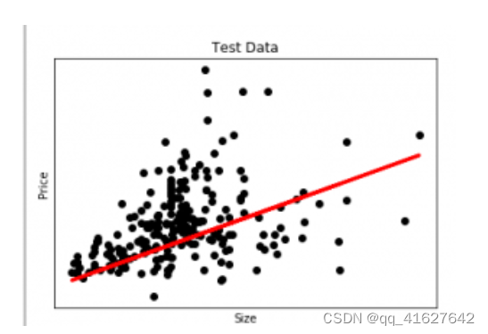
在这张图中，我们绘制了测试数据。红线表示预测价格的最佳拟合线。使用线性回归模型进行个体预测:
print( str(round(regr.predict(5000))) )

import pandas as pd
import matplotlib.pyplot as plt
import seaborn as sns
import sklearn
import warnings
 
from sklearn.preprocessing import LabelEncoder
from sklearn.impute import KNNImputer
from sklearn.model_selection import train_test_split
from sklearn.preprocessing import StandardScaler
from sklearn.metrics import f1_score
from sklearn.ensemble import RandomForestRegressor
from sklearn.ensemble import RandomForestRegressor
from sklearn.model_selection import cross_val_score
 
warnings.filterwarnings('ignore')

df= pd.read_csv('Salaries.csv')
print(df)

在这里插入图片描述
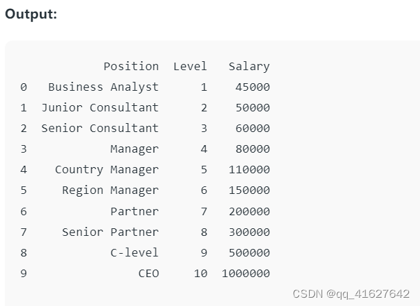
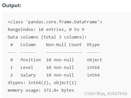
Here the .info() method provides a quick overview of the structure, data types, and memory usage of the dataset.

df.info()

在这里插入图片描述

# Assuming df is your DataFrame
X = df.iloc[:,1:2].values  #features
y = df.iloc[:,2].values  # Target variable

step 4: Random Forest Regressor model代码对分类数据进行数字编码处理，将处理后的数据与数字数据结合起来，使用准备好的数据训练Random Forest Regression模型。

import pandas as pd
from sklearn.ensemble import RandomForestRegressor
from sklearn.preprocessing import LabelEncoder
 
 Check for and handle categorical variables
label_encoder = LabelEncoder()
x_categorical = df.select_dtypes(include=['object']).apply(label_encoder.fit_transform)
x_numerical = df.select_dtypes(exclude=['object']).values
x = pd.concat([pd.DataFrame(x_numerical), x_categorical], axis=1).values
 
# Fitting Random Forest Regression to the dataset
regressor = RandomForestRegressor(n_estimators=10, random_state=0, oob_score=True)
 
# Fit the regressor with x and y data
regressor.fit(x, y)

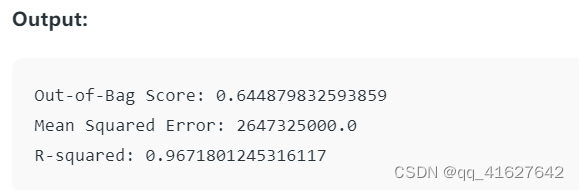
# Evaluating the model
from sklearn.metrics import mean_squared_error, r2_score
 
# Access the OOB Score
oob_score = regressor.oob_score_
print(f'Out-of-Bag Score: {oob_score}')
 
# Making predictions on the same data or new data
predictions = regressor.predict(x)
 
# Evaluating the model
mse = mean_squared_error(y, predictions)
print(f'Mean Squared Error: {mse}')
 
r2 = r2_score(y, predictions)
print(f'R-squared: {r2}')

在这里插入图片描述

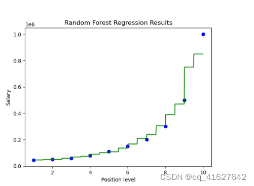
import numpy as np
X_grid = np.arange(min(X),max(X),0.01)
X_grid = X_grid.reshape(len(X_grid),1) 
   
plt.scatter(X,y, color='blue') #plotting real points
plt.plot(X_grid, regressor.predict(X_grid),color='green') #plotting for predict points
   
plt.title("Random Forest Regression Results")
plt.xlabel('Position level')
plt.ylabel('Salary')
plt.show()

在这里插入图片描述

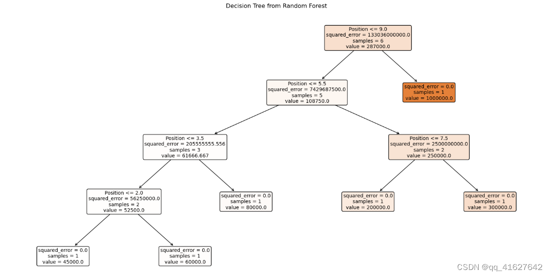
from sklearn.tree import plot_tree
import matplotlib.pyplot as plt
 
# Assuming regressor is your trained Random Forest model
# Pick one tree from the forest, e.g., the first tree (index 0)
tree_to_plot = regressor.estimators_[0]
 
# Plot the decision tree
plt.figure(figsize=(20, 10))
plot_tree(tree_to_plot, feature_names=df.columns.tolist(), filled=True, rounded=True, fontsize=10)
plt.title("Decision Tree from Random Forest")
plt.show()