7. Hierarchical Modelling

7.1 Local and world co-ordinate frames of reference

There is no (0,0,0) in the real world. Objects are always defined relative to each other. We can move (0,0,0) and thus move all the points defined relative to that origin.

7.1.1 Relative motion

A motion takes place relative to a local origin.

The term local origin refers to the (0,0,0) that is chosen to measure the motion from. The local origin may be moving relative to some greater frame of reference.

Start with a symbol (prototype). Each appearance of the object in the scene is an instance. We must scale, orient and position it to define the instance transformation

$$M=T\cdot R\cdot S$$

7.2 Linear modelling

• Copy: Creates a completely separate clone from the original. Modifying one has no effect on the other.
• Instance: Creates a completely interchangeable clone of the original. Modifying an instanced object is the same as modifying the original.
• Array: series of clones
  • Linear: Select object, Define axis, Define distance, Define number
  • Radial: Select object, Define axis, Define radius, Define number

Model stored in a table by

• assigning a number to each symbol
• storing the parameters for the instance transformation
• Contains flat information but no information on the actual structure

7.3 Hierarchical modelling

In a scene, some objects may be grouped together in some way. For example, an articulated figure may contain several rigid components connected together in a specified fashion.

Articulated model
An articulated model is an example of a hierarchical model consisting of rigid parts and connecting joints.

The moving parts can be arranged into a tree data structure if we choose some particular piece as the ‘root’.

For an articulated model (like a biped character), we usually choose the root to be somewhere near the centre of the torso.

Each joint in the figure has specific allowable degrees of freedom (DOFs) that define the range of possible poses for the model.

7.3.1 Hierarchical transformations

Each node in the tree represents an object that has a matrix describing its location and a model describing its geometry.

When a node up in the tree moves its matrix

• it takes its children with it.
• so child nodes inherit transformations from their parent node.

Each node in the tree stores a local matrix which is its transformation relative to its parent.

To compute a node’s world space matrix, we need to concatenate its local matrix with its parent’s world matrix:$$M_{world}=M_{parent}\cdot M_{local}$$

---

8. Lighting and Materials

8.1 Lighting sources

A light source can be defined with a number of properties, such as position, colour, direction, shape and reflectivity.

A single value can be assigned to each of the RGB colour components to describe the amount or intensity of the colour component.

8.1.1 Point light

This is the simplest model for an object, which emits radiant energy with a single colour specified by the three RGB components.

Large sources can be treated as point emitters if they are not too close to the scene.

The light rays are generated along radially diverging paths from the light source position.

8.1.2 Directional light

A large light source (e.g. the sun), which is very far away from the scene, can also be approximated as a point emitter, but there is little variation in its directional effects.

This is called an infinitely distant / directional light (the light beams are parallel).

一种假定离被照亮的对象有无穷远的光。从光源发出的所有光线到达场景时全是平行的。场景中每个顶点可以使用一个单独的光方向矢量。

8.1.3 Spot light

A local light source can easily be modified to produce a spotlight beam of light

If an object is outside the directional limits of the light source, it is excluded for illumination by that light source.

A spot light source can be set up by assigning a vector direction and an angular limit ${\theta }_l$ measured from the vector direction along with the position and colour.

8.2 Surface lighting effects

Although a light source delivers a single distribution of frequencies, the ambient, diffuse and specular components might be different.

8.2.1 Ambient light

The effect is a general background non-directed illumination. Each object is displayed using an intensity intrinsic to it, i.e. a world of non-reflective, self-luminous object.

Consequently each object appears as a monochromatic silhouette, unless its constituent parts are given different shades when the object is created.

The ambient component is the lighting effect produced by the reflected light from various surfaces in the scene.

When ambient light strikes a surface, it is scattered equally in all directions. The light has been scattered so much by the environment that it is impossible to determine its direction - it seems to come from all directions.

Back lighting in a room has a large ambient component, since most of the light that reaches the eye has been bounced off many surfaces first.

A spotlight outdoors has a tiny ambient component; most of the light travels in the same direction, and since it is outdoors, very little of the light reaches the eye after bouncing off other objects.

8.2.2 Diffuse reflectance

Diffuse light comes from one direction, so it is brighter if it comes squarely down on a surface than if it barely glances off the surface.

Once it hits a surface, however, it is scattered equally in all directions, so it appears equally bright, no matter where the eye is located.

Any light coming from a particular position or direction probably has a diffuse component.

Rough or grainy surfaces tend to scatter the reflected light in all directions (called diffuse reflection).

Each object is considered to present a dull, matte surface and all objects are illuminated by a point light source whose rays emanate uniformly in all directions.

The factors which affect the illumination are the point light source intensity, the material’s diffuse reflection coefficient, and the angle of incidence of the light.

8.2.3 Specular reflectance

Specular light comes from a particular direction, and it tends to bounce off the surface in a preferred direction.

A well-collimated laser beam bouncing off a high-quality mirror produces almost 100% specular reflection.

Shiny metal or plastic has a high specular component, and chalk or carpet has almost none. Specularity can be considered as shininess.

This effect can be seen on any shiny surface and the light reflected off the surface tends to have the same colour as the light source.

The reflectance tends to fall off rapidly as the viewpoint direction veers away from the direction of reflection; for perfect reflectors, specular light appears only in the direction of reflection.

8.3 Attenuation

For positional/point light sources, we consider the attenuation of light received due to the distance from the source. Attenuation is disabled for directional lights as they are infinitely far away, and it does not make sense to attenuate their intensity over distance.

Although for an ideal source the attenuation is inversely proportional to the square of the distance d, we can gain more flexibility by using the following distance-attenuation model, $$f(d)=\frac{1}{k_c+k_{l}d+k_q{d}^2}$$ where $k_c,k_l,k_q$ are three floats.

8.4 Lighting model

A lighting model (also called illumination or shading model) is used to calculate the colour of an illuminated position on the surface of an object.

The lighting model computes the lighting effects for a surface using various optical properties, which have been assigned to the surface, such as the degree of transparency, colour reflectance coefficients and texture parameters.

The lighting model can be applied to every projection position, or the surface rendering can be accomplished by interpolating colours on the surface using a small set of lighting-model calculations.

A surface rendering method uses the colour calculation from a lighting model to determine the pixel colours for all projected positions in a scene.

8.4.1 Phong model

A simple model that can be computed rapidly. Three components considered:

• Diffuse
• Specular
• Ambient

Four vectors used

• Face normal $\vec{n}$
• To viewer $\vec{v}$
• To light source $\vec{l}$
• Perfect relector $\vec{r}$

For each point light source, there are 9 coefficients $$I_{dr},I_{dg},I_{db},I_{sr},I_{sg},I_{sb},I_{ar},I_{ag},I_{ab}$$

Material properties match light source properties, there are 9 coefficients and a Shininess coefficient $\alpha$ $$k_{dr},k_{dg},k_{db},k_{sr},k_{sg},k_{sb},k_{ar},k_{ag},k_{ab}$$

For each light source and each colour component, the Phong model can be written (without the distance terms) as$$I=k_d{I}_d\vec{l}\cdot \vec{n}+k_s{I}_s(\vec{v}\cdot \vec{r}{)}^{\alpha }+k_a{I}_a$$

For each colour component, we add contributions from all sources

8.4.2 Polygonal Shading

In vertex shading, shading calculations are done for each vertex

• Vertex colours become vertex shades and can be sent to the vertex shader as a vertex attribute
• Alternately, we can send the parameters to the vertex shader and have it compute the shade

By default, vertex shades are interpolated across an object if passed to the fragment shader as a varying variable (smooth shading). We can also use uniform variables to shade with a single shade (flat shading)

8.4.3 Flat (constant) shading

If the three vectors $\vec{l},\vec{v},\vec{n}$ are constant, then the shading calculation needs to be carried out only once for each polygon, and each point on the polygon is assigned the same shade.

The polygonal mesh is usually designed to model a smooth surface, and flat shading will almost always be disappointing because we can see even small differences in shading between adjacent polygons.

8.4.4 Smooth (interpolative) shading

The rasteriser interpolates colours assigned to vertices across a polygon.

Suppose that the lighting calculation is made at each vertex using the material properties and vectors $\vec{n}$, $\vec{v}$, and $\vec{l}$ computed for each vertex. Thus, each vertex will have its own colour that the rasteriser can use to interpolate a shade for each fragment.

Note that if the light source is distant, and either the viewer is distant or there are no specular reflections, then smooth (or interpolative) shading shades a polygon in a constant colour.

FLAT与SMOOTH绘制的区别

Gouraud shading
The vertex normals are determined (average of the normals around a mesh vertex) for a polygon and used to calculate the pixel intensities at each vertex, using whatever lighting model.

Then the intensities of all points on the edges of the polygon are calculated by a process of weighted averaging (linear interpolation) of the vertex values.

The vertex intensities are linearly interpolated over the surface of the polygon.

Gouraud shading 与 Phong shading 的区别

8.5 Material colours

A lighting model may approximate a material colour depending on the percentages of the incoming red, green, and blue light reflected.

Like lights, materials have different ambient, diffuse and specular colours, which determine the ambient, diffuse and specular reflectances of the material.

The ambient reflectance of a material is combined with the ambient component of each incoming light source, the diffuse reflectance with the light’s diffuse component, and similarly for the specular reflectance component.

Ambient and diffuse reflectances define the material colour and are typically similar if not identical.

Specular reflectance is usually white or grey, so that specular highlights become the colour of the specular intensity of the light source. If a white light shines on a shiny red plastic sphere, most of the sphere appears red, but the shiny highlight is white.

8.6 RGB values for lights

The colour components specified for lights mean something different from those for materials.

• For a light, the numbers correspond to a percentage of full intensity for each colour. If the R, G and B values for a light colour are all 1.0, the light is the brightest white. If the values are 0.5, the colour is still white, but only at half intensity, so it appears grey. If R=G=1 and B=0 (full red and green with no blue), the light appears yellow.
• For materials, the numbers correspond to the reflected proportions of those colours. So if R=1, G=0.5 and B=0 for a material, the material reflects all the incoming red light, half the incoming green and none of the incoming blue light.
• In other words, if a light has components $(R_L,G_L,B_L)$, and a material has corresponding components $(R_M,G_M,B_M)$; then, ignoring all other reflectivity effects, the light that arrives at the eye is given by $(R_L\ast R_M,G_L\ast G_M,B_L\ast B_M)$.

RGB values for two lights
Similarly, if two lights, $(R_1,G_1,B_1)$ and $(R_2,G_2,B_2)$ are sent to the eye, these components are added up, giving $(R_1+R_2,G_1+G_2,B_1+B_2)$. If any of the sums are greater than 1 (corresponding to a colour brighter than the equipment can display), the component is clamped to 1.

---

9. Texture Mapping

Although graphics cards can render over 10 million polygons per second, this may be insufficient or there could be alternative way to process phenomena, e.g. clouds, grass, terrain and skin.

Although graphics cards can render over 10 million polygons per second, this may be insufficient or there could be alternative way to process phenomena, e.g. clouds, grass, terrain and skin.

What makes texture mapping tricky is that a rectangular texture can be mapped to nonrectangular regions, and this must be done in a reasonable way.

When a texture is mapped, its display on the screen might be distorted due to various transformations applied – rotations, translations, scaling and projections.

Types of texture mapping

• Texture mapping: Uses images to fill inside of polygons
• Environment (reflection) mapping: Uses a picture of the environment for texture maps. Allows simulation of highly specular surfaces.
• Bump mapping: Emulates altering normal vectors during the rendering process

9.1 Specifying the texture

There are two common types of texture:

• image: a 2D image is used as the texture.
• procedural: a program or procedure generates the texture.

The texture can be defined as one-dimensional, two-dimensional or three-dimensional patterns.

Texture functions in a graphics package often allow the number of colour components for each position in a pattern to be specified as an option.

The individual values in a texture array are often called texels (texture elements).

9.2 Magnification and minification

Depending on the texture size, the distortion and the size of the screen image, a texel may be mapped to more than one pixel (called magnification), and a pixel may be covered by multiple texels (called minification).

Since the texture is made up of discrete texels, filtering operations must be performed to map texels to pixels.

For example, if many texels correspond to a pixel, they are averaged down to fit; if texel boundaries fall across pixel boundaries, a weighted average of the applicable texels is performed.

Because of these calculations, texture mapping can be computationally expensive, which is why many specialised graphics systems include hardware support for texture mapping.

Texture mapping techniques are implemented at the end of the rendering pipeline. It is very efficient because a few polygons make it past the clipper.

9.3 Co-ordinate systems for texture mapping

• Parametric co-ordinates: may be used to model curves and surfaces
• Texture co-ordinates: used to identify points in the image to be mapped
• Object or world co-ordinates: conceptually, where the mapping takes place
• Window co-ordinates: where the final image is finally produced

9.4 Backward mapping

We really want to go backwards:

• Given a pixel, we want to know to which point on an object it corresponds.
• Given a point on an object, we want to know to which point in the texture it corresponds.

One solution to the mapping problem is to first map the texture to a simple intermediate surface.

9.4.1 First mapping

Cylindrical mapping
A parametric cylinder$$\begin{array}{rl}x& =r\cos (2\pi u)\\ y& =r\sin (2\pi u)\\ z& =vh\end{array}$$

maps a rectangle in the (u,v) space to the cylinder of radius r and height h in the world co-ordinates$$\begin{gathered} s=u \\ t=v \end{gathered}$$

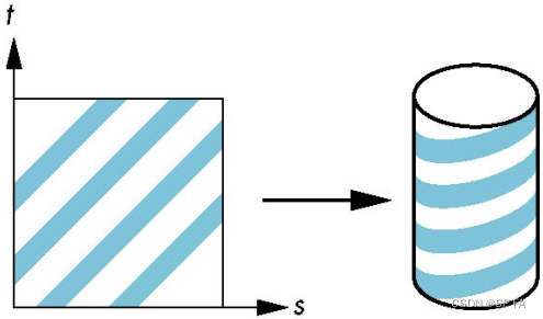
Spherical mapping
$$\begin{array}{rl}x& =r\cos (2\pi u)\\ y& =r\sin (2\pi u)\cos (2\pi v)\\ z& =r\sin (2\pi u)\sin (2\pi v)\end{array}$$

Box mapping
Easy to use with simple orthographic projection. Also used in environmental maps

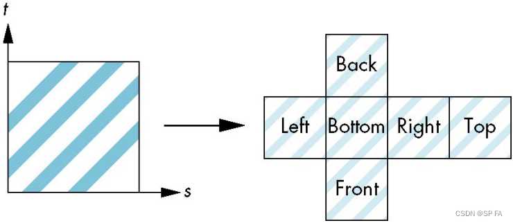
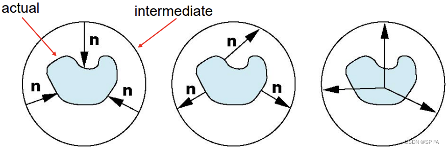
9.4.2 Second mapping

Mapping from an intermediate object to an actual object

• Normals from the intermediate to actual objects
• Normals from the actual to intermediate objects
• Vectors from the centre of the intermediate object
  

9.5 Aliasing

Point sampling of the texture can lead to aliasing errors

Area averaging
A better but slower option is to use area averaging.

10. Clipping and rasterization

Clipping: Remove objects or parts of objects that are
outside the clipping window.
Rasterization: Convert high level object descriptions to pixel colours in the framebuffer.

Why clipping
Rasterization is very expensive. Approximately linear with the number of fragments created. If we only rasterize what is actually viewable, we can save a lot of expensive computation.

Rendering pipeline

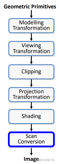
Required tasks

• Clipping
• Transformations
• Rasterization (scan conversion)
• Some tasks deferred until fragment processing
  • Hidden surface removal
  • Antialiasing

Rasterization meta algorithms
Consider two approaches to rendering a scene with opaque objects:

1. For every pixel, determine which object that projects on the pixel is closest to the viewer and compute the shade of this pixel. (Ray tracing paradigm)
2. For every object, determine which pixels it covers and shade these pixels.
   • Pipeline approach
   • Must keep track of depths

The clipping window

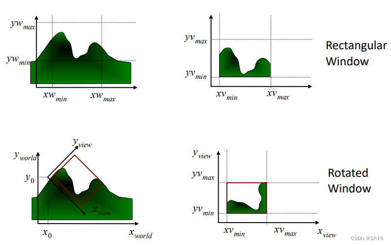
Clipping window vs viewport

• The clipping window selects what we want to see in our virtual 2D world.
• The viewport indicates where it is to be viewed on the output device (or within the display window).
• By default the viewport has the same location and dimensions of the GLUT display window we create.

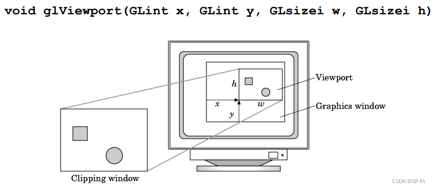
The viewport is part of the state

• changes between rendering objects or redisplay
• changes between rendering objects or redisplay

10.1 2D point clipping

Determine whether a point (x,y) is inside or outside of the window.
这个很简单。

10.2 2D line clipping

Determine whether a line is inside, outside or partially inside the window. If a line is partially inside, we need to display the inside segment.

1. Compute the line-window boundary edge intersection.
2. There will be four intersections, but only one or two are on the window edges.
3. These two points are the end points of the desired line segment.

10.2.1 Brute force clipping of lines (Simultaneous equations)

solve simultaneous equations using $y=mx+b$ for line and four clip edges

• Slope-intercept formula handles infinite lines only
• Does not handle vertical lines

10.2.2 Brute force clipping of lines (Similar triangles)

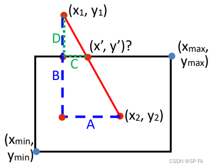
Drawbacks

• Too expensive
  • 4 floating point subtractions
  • 1 floating point multiplication
  • 1 floating point division
  • Repeat 4 times (once for each edge)

10.2.3 Cohen-Sutherland 2D line clipping

Cohen-Sutherland

• organised
• efficient
• computes new end points for the lines that must be clipped

steps

1. Creates an outcode for each end point that contains location information of the point with respect to the clipping window.
2. Uses outcodes for both end points to determine the configuration of the line with respect to the clipping window.
3. Computes new end points if necessary.
4. Extends easily to 3D (using 6 faces instead of 4 edges).

Idea: eliminate as many cases as possible without computing intersections

Start with four lines that determine the sides of the clipping window

• Case 1: both endpoints of line segment inside all four lines
• Case 2: both endpoints outside all lines and on same side of a line
• Case 3: One endpoint inside, one outside (Must do at least one intersection)
• Case 4: Both outside (May have part inside, must do at least one intersection)

defining outcodes

1. Split plane into 9 regions.
2. Assign each a 4-bit outcode (above, below, right and left).
3. Assign each endpoint an outcode.

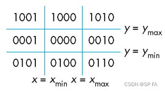
Efficiency
In many applications, the clipping window is small relative to the size of the entire database.

Most line segments are outside one or more sides of the window and can be eliminated based on their outcodes.

Inefficient when code has to be re-executed for line segments that must be shortened in more than one step, because two intersections have to be calculated anyway, in addition to calculating the outcode (extra computing in such a case).

10.2.4 Cohen-Sutherland 3D line clipping

Use 6-bit outcodes, when needed, clip line segment against planes

10.2.5 Liang-Barsky (Parametric line formulation)

Consider the parametric form of a line segment$$p(\alpha )=(1-\alpha ){\vec{p}}_1+\alpha {\vec{p}}_2,0\le \alpha \le 1$$ We can distinguish the cases by looking at the ordering of the $\alpha$ values where the line is determined by the line segment crossing the lines that determine the window.

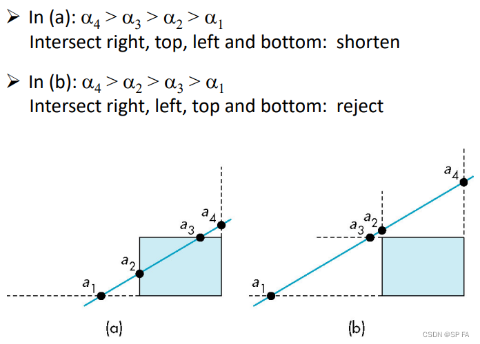
Advantages:

• Can accept/reject as easily as with Cohen-Sutherland
• Using values of $\alpha$, we do not have to use the algorithm recursively as with the Cohen-Sutherland method
• easily Extends to 3D

10.3 Plane-line intersections

If we write the line and plane equations in matrix form (where $n$ is the normal to the plane and $p_0$ is a point on the plane), we must solve the equations.$$\vec{n}\cdot (p(\alpha )-{\vec{p}}_0)=0$$For the $\alpha$ corresponding to the point of intersection, this value is$$\alpha =\frac{\vec{n}\cdot ({\vec{p}}_0-{\vec{p}}_1)}{\vec{n}\cdot ({\vec{p}}_2-{\vec{p}}_1)}$$The intersection requires 6 multiplications and 1 division.

General 3D clipping
General clipping in 3D requires intersection of line segments against arbitrary plane.

Normalised form
Normalisation is part of viewing (pre clipping) but after normalisation, we clip against sides of right parallelepiped.

10.4 Polygon clipping

Not as simple as line segment clipping

• Clipping a line segment yields at most one line segment
• Clipping a polygon can yield multiple polygons

However, clipping a convex polygon can yield at most one other polygon.

10.4.1 Convexity and tessellation

One strategy is to replace non-convex (concave) polygons with a set of triangular polygons (a tessellation). It also makes fill easier.

10.4.2 Clipping as a black box

We can consider line segment clipping as a process that takes in two vertices and produces either no vertices or the vertices of a clipped line segment.

Pipeline clipping of line segments
Clipping against each side of window is independent of other sides so we can use four independent clippers in a pipeline.

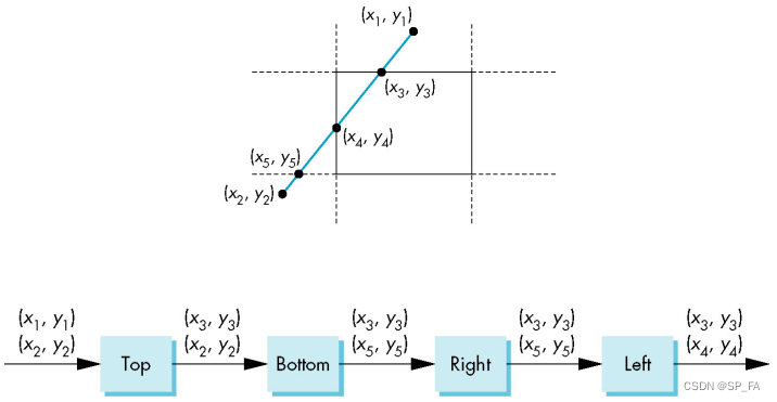
Pipeline clipping of polygons
add front and back clippers (Strategy used in SGI Geometry Engine)

10.4.3 Bounding boxes

Rather than doing clipping on a complex polygon, we can use an axis-aligned bounding box or extent:

• Smallest rectangle aligned with axes that encloses the polygon

10.5 Other issues in clipping

• Clipping other shapes: Circle, Ellipse, Curves
• Clipping a shape against another shape.
• Clipping the interior

---

11. Hidden Surface Removal

Clipping has much in common with hidden-surface removal. In both cases, we try to remove objects that are not visible to the camera.

Often we can use visibility or occlusion testing early in the process to eliminate as many polygons as possible before going through the entire pipeline.

Object space algorithms: determine which objects are in front of others.

• Resize does not require recalculation
• Works for static scenes
• May be difficult / impossible to determine

Image space algorithms: determine which object is visible at each pixel

• Resize requires recalculation
• Works for dynamic scenes

11.1 Painter’s algorithm

It is an object-space algorithm. Render polygons in the back to front order so that polygons behind others are simply painted over.

Sort surfaces/polygons by their depth (z value). Not every polygon is either in front or behind all other polygons.

• Polygon $A$ lies entirely behind all other polygons, and can be painted first.
• Polygons which overlap in $z$ but not in either $x$ or $y$, can be painted independently.
• Hard cases: Overlap in all directions (polygons with overlapping projections)

11.2 Back-face culling

Back-face culling is the process of comparing the position and orientation of polygons against the viewing direction $\vec{v}$, with polygons facing away from the camera eliminated.

This elimination minimises the amount of computational overhead involved in hidden-surface removal.

Back-face culling is basically a test for determining the visibility of a polygon, and based on this test the polygon can be removed if not visible – also called back-surface removal.

For each polygon $P_i$

• Find polygon normal $\vec{n}$
• Find viewer direction $\vec{v}$
• if $\vec{v}\cdot \vec{n}<0$, then cull $P_i$

Back-face culling does not work for:

• Overlapping front faces due to multiple objects or concave objects
• Non-polygonal models
• Non-closed Objects

11.3 Image space approach

Look at each projector ($n\ast m$ projectors for an $n\ast m$ framebuffer) and find the closest among $k$ polygons.

11.3.1 Z-buffer

We now know which pixels contain which objects; however since some pixels may contain two or more objects, we must calculate which of these objects are visible and which are hidden.

In graphics hardware, hidden-surface removal is generally accomplished using the Z-buffer algorithm.

we set aside a two-dimensional array of memory (the Z-buffer) of the same size as the screen (number of rows * number of columns). This is in addition to the colour buffer. The Z-buffer will hold values which are depths (quite often z-values). The Z-buffer is initialised so that each element has the value of the far clipping plane (the largest possible z-value after clipping is performed). The colour buffer is initialised so that each element contains a value which is the background colour.

Now for each polygon, we have a set of pixel values which the polygon covers. For each of the pixels, we compare its depth (z-value) with the value of the corresponding element already stored in the Z-buffer:

• If this value is less than the previously stored value, the pixel is nearer the viewer than the previously encountered pixel;
• Replace the value of the Z- buffer with the z value of the current pixel, and replace the value of the colour buffer with the value of the current pixel.

Repeat for all polygons in the image. The implementation is typically done in normalised co-ordinates so that depth values range from 0 at the near clipping plane to 1.0 at the far clipping plane.

Advantages

• The most widely used hidden-surface removal algorithm
• Relatively easy to implement in hardware or software
• An image-space algorithm which traverses scene and operates per polygon rather than per pixel
• We rasterize polygon by polygon and determine which (part of) polygons get drawn on the screen.

Memory requirements

• Relies on a secondary buffer called the Z-buffer or depth buffer
• Z-buffer has the same width and height as the framebuffer
• Each cell contains the z-value (distance from viewer) of the object at that pixel position.

11.3.2 Scan-line

If we work scan line by scan line as we move across a scan line, the depth changes satisfy $a\Delta x+b\Delta y+c\Delta z=0$, noticing that the plane which contains the olygon is represented by $ax+by+cz+d=0$

• Worst-case performance of an image-space algorithm is proportional to the number of primitives
• Performance of z-buffer is proportional to the number of fragments generated by rasterization, which depends on the area of the rasterized polygons.

We can combine shading and hidden-surface removal through scan line algorithm.

• Scan line i: no need for depth information, can only be in no or one polygon.
• Scan line j: need depth information only when in more than one polygon.
  

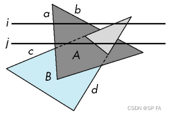
implementation

• Flag for each polygon (inside/outside)
• Incremental structure for scan lines that stores which edges are encountered
• Parameters for planes

11.3.3 BSP tree

In many real-time applications, such as games, we want to eliminate as many objects as possible within the application so that we can

• reduce burden on pipeline
• reduce traffic on bus

Partition space with Binary Spatial Partition (BSP) Tree

Consider 6 parallel planes. Plane A separates planes B and C from planes D, E and F.

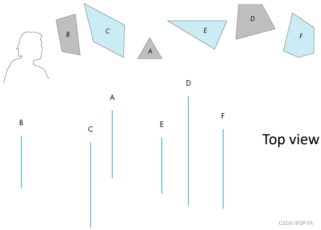
We can put this information in a BSP tree. Use the BSP tree for visibility and occlusion testing.

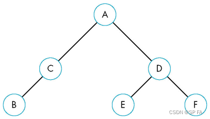
The painter’s algorithm for hidden-surface removal works by drawing all faces, from back to front.

constructing

1. Choose polygon (arbitrary)
2. Split the cell using the plane on which the polygon lies (May have to clip)
3. Continue until each cell contains only one polygon fragment
4. Splitting planes could be chosen in other ways, but there is no efficient optimal algorithm for building BSP trees
   • BSP trees are not unique, there can be a number of alternatives for the same set of polygons
   • Optimal means minimum number of polygon fragments in a balanced tree

Rendering
The rendering is recursive descent of the BSP tree.

At each node (for back to front rendering):

• Recurse down the side of the sub-tree that does not contain the viewpoint. Test viewpoint against the split plane to decide the polygon.
• Draw the polygon in the splitting plane. Paint over whatever has already been drawn.
• Recurse down the side of the tree containing the viewpoint