🧑‍💻 本文主要讲解Megatron早期版本中的数据混合算法。

1. 数据混合

在谈源码之前，我们有必要先了解一下Megatron中的数据混合思想。

给定 $n$ 个数据集 ${\mathcal{D}}_1,{\mathcal{D}}_2,\cdots ,{\mathcal{D}}_n$ 和对应的 $n$ 个权重 $w_1,w_2,\cdots ,w_n$，我们要按照这些权重去混合 $n$ 个数据集，设混合后的数据集为 $\mathcal{D}$。

Megatron假定：

• $|\mathcal{D}|={\sum }_{i=1}^n|{\mathcal{D}}_i|$。即混合后的数据集大小等于混合前的各数据集大小之和。
• $\mathcal{D}$ 中有约 $|\mathcal{D}|\cdot w_i$ 个样本来自 ${\mathcal{D}}_i$。

那如何确定 $\mathcal{D}$ 中到底有多少个样本是来自 ${\mathcal{D}}_i$ 的呢？一种最直观的做法是，计算 $|\mathcal{D}|\cdot w_i$，然后进行取整，但这种操作无法保证所有取整后的 $|\mathcal{D}|\cdot w_i$ 相加起来恰好是 $|\mathcal{D}|$。 如果总和大于 $|\mathcal{D}|$，说明某些数据集被过采样了，应当减少相应数据集的采样数；如果总和小于 $|\mathcal{D}|$，说明某些数据集被欠采样了，应当增加相应数据集的采样数。可问题是，如何确定这些被过采样/欠采样的数据集呢？显然我们需要一个更加公平的算法。

我们可以把获取数据集 $\mathcal{D}$ 看作是一个采样过程：一开始有 $n$ 个数据源 { D i } i = 1 n \{\mathcal{D}_i\}_{i=1}^n {Di​}i=1n​，每一轮迭代，我们需要先从这 $n$ 个数据源中选出一个数据源 ${\mathcal{D}}_i$，然后再从这个数据源中选出一个样本 $\mathcal{S}$。 由于每一轮迭代只会选出一个样本，因此 $|\mathcal{D}|$ 轮迭代结束后，我们便得到了 $|\mathcal{D}|$ 个样本，这些样本构成了混合后的数据集 $\mathcal{D}$。

每一轮迭代都会产生两个信息：要选取的数据源 ${\mathcal{D}}_i$，要从 ${\mathcal{D}}_i$ 中选取的样本。我们可以考虑构造两个整数序列 $\mathcal{P},\mathcal{S}$，它们的长度均为 $|\mathcal{D}|$，含义如下：

• ${\mathcal{P}}_j$ 代表的是第 $j$ 轮迭代时，选取的数据源的下标。例如 ${\mathcal{P}}_{10}=3$ 意味着第 $10$ 轮迭代选取的数据源是 ${\mathcal{D}}_3$。
• ${\mathcal{S}}_j$ 代表的是第 $j$ 轮迭代时，从数据源 ${\mathcal{D}}_{{\mathcal{P}}_j}$ 选取的样本的下标。

由以上定义知，$\forall j$，都有 $1\le {\mathcal{P}}_j\le n$，$1\le {\mathcal{S}}_j\le |{\mathcal{D}}_{{\mathcal{P}}_j}|$（下标均从 $1$ 开始）。

接下来的问题是，如何确定每一轮的 ${\mathcal{P}}_j$ 和 ${\mathcal{S}}_j$ 呢？

先谈 ${\mathcal{P}}_j$。因为是一个从 $1$ 到 $|\mathcal{D}|$ 的一个逐步采样过程，在第 $j$ 轮迭代时，我们已经抽取了 $j-1$ 个样本，接下来要确定第 $j$ 个样本。根据Megatron的假定，在确定下来第 $j$ 个样本后，这 $j$ 个样本中应当有约 $j\cdot w_i$ 个样本是来自 ${\mathcal{D}}_i$ 的。

考虑构造一个长度为 $n$ 的序列 $\mathcal{C}$，该序列随着迭代不断更新。${\mathcal{C}}_i$ 代表当前已经从 ${\mathcal{D}}_i$ 抽取了多少个样本。显然可知，第一轮迭代开始时，有 ${\mathcal{C}}_i=0,i=1,2,\cdots ,n$。最后一轮迭代结束后，有 ${\sum }_{i=1}^n{\mathcal{C}}_i=|\mathcal{D}|$，并且

$${\mathcal{C}}_i=\{\begin{array}{ll}{\sum }_{t=1}^{j-1}I({\mathcal{P}}_t=i),& \text{Pj确定前}\\ {\sum }_{t=1}^{j}I({\mathcal{P}}_t=i),& \text{Pj确定后}\end{array},\forall i$$

回到对 ${\mathcal{P}}_j$ 的讨论中。假设在确定第 $j$ 个样本前已经从 ${\mathcal{D}}_i$ 中抽取了 ${\mathcal{C}}_i$ 个样本，在确定第 $j$ 个样本后，诸 ${\mathcal{C}}_i$ 中有且仅有一个的值会增加 $1$，不妨记为 ${\mathcal{C}}_k$，这个过程可以形容为

$$\underset{第j轮迭代开始时}{\underbrace{[{\mathcal{C}}_1,\cdots ,{\mathcal{C}}_k,\cdots ,{\mathcal{C}}_n]}}\to \underset{第j轮迭代结束时}{\underbrace{[{\mathcal{C}}_1,\cdots ,{\mathcal{C}}_k+1,\cdots ,{\mathcal{C}}_n]}}\underset{理论值}{\underbrace{[j\cdot w_1,j\cdot w_2,\cdots ,j\cdot w_n]}}$$

我们期望第 $j$ 轮迭代结束时，诸 ${\mathcal{C}}_i$ 应当尽可能地接近理论值（在MSE下）。由于只能让其中一个 ${\mathcal{C}}_k$ 自增 $1$，显然有 $k={\mathrm{argmax}}_i(j\cdot w_i-{\mathcal{C}}_i)$。

再谈 ${\mathcal{S}}_j$。在确定了数据源是 ${\mathcal{D}}_k$ 后，为了避免重复，我们应当做到不放回、随机地从中采样。如何做到这两点呢？我们可以在一开始就对 $n$ 个数据源进行打乱，然后在采样的时候只需要从前往后进行，就可以做到以上两点。注意到 ${\mathcal{C}}_i$ 的值是从 $0$ 开始，以步长为 $1$ 依次递增，所以我们可以用每次更新完的 ${\mathcal{C}}_i$ 赋值给相应的 ${\mathcal{S}}_j$，即 ${\mathcal{S}}_j=第j轮迭代结束时的{\mathcal{C}}_i$。

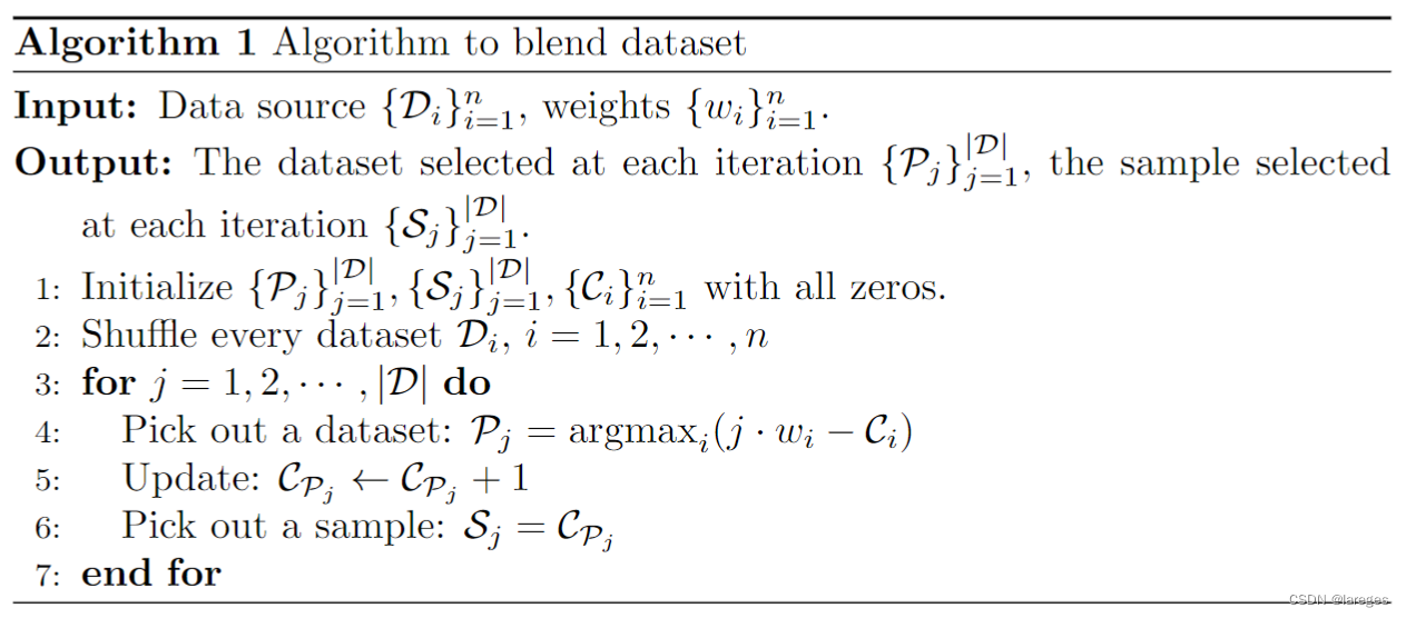
由此我们可以得到整个算法的伪代码：

2. 源码解析

Python部分：

class BlendableDataset(torch.utils.data.Dataset):
    def __init__(self, datasets, weights):
        self.datasets = datasets
        num_datasets = len(datasets)
        assert num_datasets == len(weights), "The number of datasets and weights must match."

        self.size = sum(len(dataset) for dataset in self.datasets)

        # Normalize weights.
        weights = np.array(weights, dtype=np.float64)
        sum_weights = np.sum(weights)
        assert sum_weights > 0.0, "Sum of weights must be positive."
        weights /= sum_weights

        # Build indices.
        start_time = time.time()
        assert num_datasets < 255, "Number of datasets must be less than 255."
        self.dataset_index = np.zeros(self.size, dtype=np.uint8)
        self.dataset_sample_index = np.zeros(self.size, dtype=np.int64)

        helpers.build_blending_indices(
            self.dataset_index,
            self.dataset_sample_index,
            weights,
            num_datasets,
            self.size,
            torch.distributed.get_rank() == 0,
        )
        print_rank_0(f'> elapsed time for building blendable dataset indices: '
                     f'{time.time() - start_time:.2f} sec')

    def __len__(self):
        return self.size

    def __getitem__(self, idx):
        dataset_idx = self.dataset_index[idx]
        sample_idx = self.dataset_sample_index[idx]
        return {
            "dataset_idx": dataset_idx,
            **self.datasets[dataset_idx][sample_idx],
        }

C++部分：

void build_blending_indices(
    py::array_t<uint8_t> &dataset_index,
    py::array_t<int64_t> &dataset_sample_index,
    const py::array_t<double> &weights,
    const int32_t num_datasets,
    const int64_t size,
    const bool verbose
) {
    /* Given multiple datasets and a weighting array, build samples
       such that it follows those weights. */

    if (verbose) {
        std::cout << "> building indices for blendable datasets ..." << std::endl;
    }

    // Get the pointer access without the checks.
    auto dataset_index_ptr = dataset_index.mutable_unchecked<1>();
    auto dataset_sample_index_ptr = dataset_sample_index.mutable_unchecked<1>();
    auto weights_ptr = weights.unchecked<1>();

    // Initialize buffer for number of samples used for each dataset.
    int64_t current_samples[num_datasets];
    for (int64_t i = 0; i < num_datasets; ++i) {
        current_samples[i] = 0;
    }

    // For each sample:
    for (int64_t sample_idx = 0; sample_idx < size; ++sample_idx) {

        // Determine where the max error in sampling is happening.
        auto sample_idx_double = std::max(static_cast<double>(sample_idx), 1.0);
        int64_t max_error_index = 0;
        double max_error = weights_ptr[0] * sample_idx_double - static_cast<double>(current_samples[0]);
        for (int64_t dataset_idx = 1; dataset_idx < num_datasets; ++dataset_idx) {
            double error = weights_ptr[dataset_idx] * sample_idx_double - static_cast<double>(current_samples[dataset_idx]);
            if (error > max_error) {
                max_error = error;
                max_error_index = dataset_idx;
            }
        }

        // Populate the indices.
        dataset_index_ptr[sample_idx] = static_cast<uint8_t>(max_error_index);
        dataset_sample_index_ptr[sample_idx] = current_samples[max_error_index];

        // Update the total samples.
        current_samples[max_error_index] += 1;
    }

    // Print info
    if (verbose) {
        std::cout << " > sample ratios:" << std::endl;
        for (int64_t dataset_idx = 0; dataset_idx < num_datasets; ++dataset_idx) {
            auto ratio = static_cast<double>(current_samples[dataset_idx]) / static_cast<double>(size);
            std::cout << "   dataset " << dataset_idx << ", input: " << weights_ptr[dataset_idx] << ", achieved: " << ratio << std::endl;
        }
    }
}

---

具体的算法实现是在C++的函数中，我们先来看Python部分。

self.size 实际上就是 $|\mathcal{D}|$，即混合后的数据集大小（从后面的 __len__ 也能看出）。在构造函数中，首先会对 weights 进行归一化，然后声明 $\mathcal{P},\mathcal{S}$ 两个数组。注意 self.dataset_index 实际上就是 $\mathcal{P}$，self.dataset_sample_index 实际上就是 $\mathcal{S}$。由于 $\mathcal{P}$ 的数据类型是 uint8，这表明其中元素的范围是 $[0,2^8-1=255]$，故 $\mathcal{P}$ 最多能表示 $256$ 个数据集，而源码中规定了参与混合的数据集个数必须严格少于 $255$（博主不是很懂这一点，看懂的小伙伴可以在评论区留言）。

再来看C++部分。前五个形参分别是 P , S , { w i } i , n , ∣ D ∣ \mathcal{P},\mathcal{S},\{w_i\}_i,n,|\mathcal{D}| P,S,{wi​}i​,n,∣D∣。

$\mathcal{C}$ 数组会在该函数中进行声明并初始化。随后的两个嵌套 for 循环则是整个算法的核心流程，注意到这里的实现中，sample_idx（即 $j$）是从 $0$ 开始的，而算法伪代码中的 $j$ 是从 $1$ 开始的，所以一开始要执行 $j=\max (j,1)$ 以确保 $j$ 至少是 $1$（但这样做有一个弊端就是前两轮的循环里，$j$ 的值是相同的，和我们期望的每一轮里 $j$ 值不同相违背，这是源码中的一个缺陷，实际上应该计算 $(j+1)\cdot w_i-{\mathcal{C}}_i$）。内层循环中的 error 实际上就是 $j\cdot w_i-{\mathcal{C}}_i$。此外，由于 $j$ 是从 $0$ 开始的，所以 ${\mathcal{C}}_{{\mathcal{P}}_j}$ 的更新要放到最后执行。

一言以蔽之，$j$ 从 $1$ 开始，更新顺序为 $\mathcal{P}\to \mathcal{C}\to \mathcal{S}$；$j$ 从 $0$ 开始，更新顺序为 $\mathcal{P}\to \mathcal{S}\to \mathcal{C}$。

得到了 $\mathcal{P},\mathcal{S}$ 数组后，我们便可得到混合后的数据集 $\mathcal{D}$：

$${\mathcal{D}}_j={\mathcal{D}}_{{\mathcal{P}}_j}[{\mathcal{S}}_j],j=1,2,\cdots ,|\mathcal{D}|$$

其中 ${\mathcal{D}}_i[j]$ 代表数据集 ${\mathcal{D}}_i$ 中的第 $j$ 个样本。

回到Python部分，__getitem__ 中传入的 idx 实际上就是 $j$，self.datasets[dataset_idx][sample_idx] 实际上就是上述的 ${\mathcal{D}}_{{\mathcal{P}}_j}[{\mathcal{S}}_j]$。

3. 证明部分&讨论

---

$\text{Prop}1.$ 每一轮循环开始时所有误差加和为 $1$，即 ${\sum }_{i=1}^n{e}_i=1$，其中 $e_i\triangleq j\cdot w_i-{\mathcal{C}}_i$。

$Proof.$ 注意到第 $j$ 轮循环开始时，此时一共只采样了 $j-1$ 个样本，所以 ${\sum }_{i=1}^n{\mathcal{C}}_i=j-1$，从而

$$\sum _{i=1}^n{e}_i=\sum _{i=1}^n(j\cdot w_i-{\mathcal{C}}_i)=j\cdot \sum _{i=1}^n{w}_i-\sum _{i=1}^n{\mathcal{C}}_i=j-\sum _{i=1}^n{\mathcal{C}}_i=j-(j-1)=1$$

进一步可知，每一轮循环结束时所有误差加和为 $0$。

---

$\text{Prop}2.$ 假定下标从 $1$ 开始，且 $n=2$（即只有两个数据源）。若 $e_1\ge 0.5$，则 ${\mathcal{P}}_j=1$，否则 ${\mathcal{P}}_j=2$。

$Proof.$ $e_1>0.5$ 的情况显然。当 $e_1=e_2=0.5$ 时，$\mathrm{argmax}$ 会优先挑选下标最小的，故此时 ${\mathcal{P}}_j$ 仍是 $1$。

---

$\text{Prop}3.$ 假定下标从 $1$ 开始。可能存在一组 { D i } i \{\mathcal{D}_i\}_i {Di​}i​ 和 { w i } i \{w_i\}_i {wi​}i​，使得经由上述算法得到的 $\mathcal{P},\mathcal{S}$ 数组，$\exists j,\text{s.t.}{\mathcal{S}}_j>|{\mathcal{D}}_{{\mathcal{P}}_j}|$，意味着 __getitem__ 会出现下标越界的错误。

$Proof.$ 构造特殊情形即可。令 $n=2$，$|{\mathcal{D}}_1|=|{\mathcal{D}}_2|=2$，$w_1=0.1,w_2=0.9$。

由 $|{\mathcal{D}}_1|+|{\mathcal{D}}_2|=4$ 可知，总共会有 $4$ 轮循环。且理应有 $1\le {\mathcal{P}}_j,{\mathcal{S}}_j\le 2,j=1,2,3,4$。

利用 $\text{Prop}2$ 快速计算：

• 第一轮循环，计算误差 $e_1=1\cdot w_1-0=0.1<0.5$，故 ${\mathcal{P}}_1=2$， C = { 0 , 1 } \mathcal{C}=\{0,1\} C={0,1}，${\mathcal{S}}_1={\mathcal{C}}_2=1$。

• 第二轮循环，计算误差 $e_1=2\cdot w_1-0=0.2<0.5$，故 ${\mathcal{P}}_2=2$， C = { 0 , 2 } \mathcal{C}=\{0,2\} C={0,2}，${\mathcal{S}}_2={\mathcal{C}}_2=2$。

• 第三轮循环，计算误差 $e_1=3\cdot w_1-0=0.3<0.5$，故 ${\mathcal{P}}_3=2$， C = { 0 , 3 } \mathcal{C}=\{0,3\} C={0,3}，${\mathcal{S}}_3={\mathcal{C}}_2=3$。

• 第四轮循环，计算误差 $e_1=4\cdot w_1-0=0.4<0.5$，故 ${\mathcal{P}}_4=2$， C = { 0 , 4 } \mathcal{C}=\{0,4\} C={0,4}，${\mathcal{S}}_4={\mathcal{C}}_2=4$。

由上可知 $j=3,4$ 满足要求。

---

$\text{Prop}4.$ 在MSE下，要使 $[{\mathcal{C}}_1,\cdots ,{\mathcal{C}}_k+1,\cdots ,{\mathcal{C}}_n]$ 尽可能接近 $[j\cdot w_1,j\cdot w_2,\cdots ,j\cdot w_n]$，应当有 $k={\mathrm{argmax}}_i(j\cdot w_i-{\mathcal{C}}_i)$。

$Proof.$ 注意到

$$\begin{array}{rl}\Delta \text{MSE}={\text{MSE}}_{after}-{\text{MSE}}_{before}& =\frac{1}{n}[(j\cdot w_k-{\mathcal{C}}_k-1{)}^2-(j\cdot w_k-{\mathcal{C}}_k{)}^2]\\ & =\frac{1}{n}[1-2(j\cdot w_k-{\mathcal{C}}_k)]\end{array}$$

由上式可知，要使 $\Delta \text{MSE}$ 越小，应使 $j\cdot w_k-{\mathcal{C}}_k$ 越大，故 $k={\mathrm{argmax}}_i(j\cdot w_i-{\mathcal{C}}_i)$。

---

$\text{Prop}5.$ 假定下标从 $1$ 开始。若 $w_1=w_2=\cdots =w_n=1/n$，令 $|\mathcal{D}|=q\cdot n+r$，其中 $q$ 是商，$r$ 是余数，则有

$$\begin{array}{rl}\mathcal{P}& =[1,2,\cdots ,n]\ast q+[1,2,\cdots ,r]\\ \mathcal{S}& =\underset{每个列表的长度均为n}{\underbrace{[1,1,\cdots ,1]+[2,2,\cdots ,2]+\cdots +[q,q,\cdots ,q]}}+\underset{长度为r}{\underbrace{[q+1,q+1,\cdots ,q+1]}}\\ \mathcal{C}& =[\underset{r个}{\underbrace{q+1,q+1,\cdots ,q+1}},\underset{n-r个}{\underbrace{q,q,\cdots ,q}}]\end{array}$$

上述的 $\ast$ 和 $+$ 均是列表运算符。

$Proof.$ 证明留给读者。

---

讨论：

$\text{Prop}3.$ 中提到了可能会出现下标越界的错误，为了避免这个错误，我们可以在得到 $\mathcal{P},\mathcal{S}$ 数组后，对 $\mathcal{S}$ 进行更新（假定下标从 $1$ 开始）：

$${\mathcal{S}}_j={\mathcal{S}}_j\text{mod}(|{\mathcal{D}}_{{\mathcal{P}}_j}|+1),j=1,2,\cdots ,|\mathcal{D}|$$

例如某个数据集是 $[1,2,3,4,5]$，如果要从这个数据集采样 $8$ 个样本，则原先的算法会在采样第 $6$ 个样本时抛出下标越界错误，修正后的算法的采样结果为 $[1,2,3,4,5,1,2,3]$。

为什么Megatron源码里没有规避这个错误但在使用的过程中却好像并没有遇到bug呢？注意到 self.datasets[dataset_idx] 实际上指向的是 megatron/data/gpt_dataset.py 中的 GPTDataset 类，在混合数据集场景下，Megatron会预先根据权重计算每个数据集所需要的样本数，然后根据这个样本数构建 GPTDataset，而非根据document数去构建。所以，即使对于两个完全相同的数据集，当赋予它们的权重不同时，所得到的 GPTDataset 的长度也不同，这一点可以通过向 BlendableDataset 源码中加入以下代码来验证：

for i, dataset in enumerate(self.datasets):
    print(f"dataset {i}: {len(dataset)}")

因为 GPTDataset 的长度已经根据权重做出了相应的调整，所以绝大部分时候是不会出现bug的，但我们依然可以构造极端情形来触发bug。

考虑在训练脚本中提供两个完全相同的路径，但却赋予它们不同的权重，如下：

--train-data-path 0.001 /path/to/your/data_text_document 0.999 /path/to/your/data_text_document

然后在 BlendableDataset 源码中的 __getitem__ 方法中固定索引，即：

def __getitem__(self, idx):
	idx = self.size - 1  # 意味着我们总是取BlendableDataset的最后一个样本
    dataset_idx = self.dataset_index[idx]
    sample_idx = self.dataset_sample_index[idx]
    return {
        "dataset_idx": dataset_idx,
        **self.datasets[dataset_idx][sample_idx],
    }

这样就可以稳定的触发下标越界的bug。

📝 注意到从 GPTDataset 中取出来的是sample，所以Megatron的混合算法实际上是以sample为单位的，而非以document为单位。

4. 进一步优化

根据 $\text{Prop}3.$ 和 $\text{Prop}5.$ 以及其他细节，我们有以下几个优化方向：

• 修复可能会出现的下标越界错误（可通过取余来实现）。
• 在等权重情形下加速混合（利用 numpy）。
• 支持更多数据集进行混合（修改 uint8 为其他类型）。

假设相应的接口名为 make_blendable_dataset，它接收两个形参：datasets 和 weights。前者是一个二维列表，包含了要进行混合的数据集（每个数据集是一个一维列表），后者是一个一维列表，包含了每个数据集的权重。

使用Python进行实现：

from typing import List, Any, Union
import numpy as np
import random
from tqdm import tqdm

def make_blendable_dataset(datasets: List[List[Any]], weights: List[Union[float, int]]) -> List[Any]:
    num_datasets = len(datasets)
    assert num_datasets == len(weights), "The number of datasets must match the number of weights."

    # Shuffle
    size = 0
    for dataset in datasets:
        size += len(dataset)
        random.shuffle(dataset)

    # Normalize weights
    weights = np.array(weights, dtype=np.float64)
    assert np.all(weights > 0), "All weights must be positive."
    weights /= weights.sum()

    # Determine if all weights are equal
    if np.ptp(weights) < 1e-5:
        q, r = divmod(size, num_datasets)
        dataset_index = np.concatenate([
            np.tile(np.arange(num_datasets, dtype=np.int16), q),
            np.arange(r, dtype=np.int16)
        ])
        dataset_sample_index = np.concatenate([
            np.repeat(np.arange(q, dtype=np.int64), num_datasets),
            np.full(r, q, dtype=np.int64)
        ])
        current_samples = np.full(num_datasets, q, dtype=np.int64)
        current_samples[:r] += 1
    else:
        dataset_index = np.zeros(size, dtype=np.int16)
        dataset_sample_index = np.zeros(size, dtype=np.int64)
        current_samples = np.zeros(num_datasets, dtype=np.int64)

        for sample_idx in tqdm(range(size), desc="Calculating error"):
            errors = weights * (sample_idx + 1) - current_samples
            max_error_index = np.argmax(errors)
            dataset_index[sample_idx] = max_error_index
            dataset_sample_index[sample_idx] = current_samples[max_error_index]
            current_samples[max_error_index] += 1

    print(f"Ratios:")
    for i in range(num_datasets):
        print(f"input: {weights[i]}, achieved: {current_samples[i] / size}")

    # Blend
    res = []
    for i in tqdm(range(size), desc="Blending"):
        dataset_idx = dataset_index[i]
        sample_idx = dataset_sample_index[i] % len(datasets[dataset_idx])
        res.append(datasets[dataset_idx][sample_idx])

    return res