目录
背影
摘要
随机森林的基本定义
随机森林实现的步骤
基于随机森林的回归分析
随机森林回归分析完整代码及工具箱下载链接: 随机森林分类工具箱,分类随机森林,随机森林回归工具箱,回归随机森林资源-CSDN文库 https://download.csdn.net/download/abc991835105/88137234
效果图
结果分析
展望
参考论文
背影
传统的回归分析一般用最小二乘等进行拟合,局部优化能力有限,本文用随机森林进行回归分析,利用每个树的增强局部优化,从而更好的拟合自变量与因变量的关系,实现回归分析的提高
摘要
LSTM原理,MATALB编程长短期神经网络LSTM的飞行轨迹预测。
随机森林的基本定义
在机器学习中,随机森林是一个包含多个决策树的分类器, 并且其输出的类别是由个别树输出的类别的众数而定。 Leo Breiman和Adele Cutler发展出推论出随机森林的算法。 而 “Random Forests” 是他们的商标。 这个术语是1995年由贝尔实验室的Tin Kam Ho所提出的随机决策森林(random decision forests)而来的。这个方法则是结合 Breimans 的 “Bootstrap aggregating” 想法和 Ho 的"random subspace method"以建造决策树的集合。
训练方法
根据下列算法而建造每棵树 [1] :
用N来表示训练用例(样本)的个数,M表示特征数目。
输入特征数目m,用于确定决策树上一个节点的决策结果;其中m应远小于M。
从N个训练用例(样本)中以有放回抽样的方式,取样N次,形成一个训练集(即bootstrap取样),并用未抽到的用例(样本)作预测,评估其误差。
对于每一个节点,随机选择m个特征,决策树上每个节点的决定都是基于这些特征确定的。根据这m个特征,计算其最佳的分裂方式。
每棵树都会完整成长而不会剪枝,这有可能在建完一棵正常树状分类器后会被采用)
随机森林的优缺点
随机森林的优点有 [2] :
1)对于很多种资料,它可以产生高准确度的分类器;
2)它可以处理大量的输入变数;
3)它可以在决定类别时,评估变数的重要性;
4)在建造森林时,它可以在内部对于一般化后的误差产生不偏差的估计;
5)它包含一个好方法可以估计遗失的资料,并且,如果有很大一部分的资料遗失,仍可以维持准确度;
6)它提供一个实验方法,可以去侦测variable interactions;
7)对于不平衡的分类资料集来说,它可以平衡误差;
8)它计算各例中的亲近度,对于数据挖掘、侦测离群点(outlier)和将资料视觉化非常有用;
9)使用上述。它可被延伸应用在未标记的资料上,这类资料通常是使用非监督式聚类。也可侦测偏离者和观看资料;
10)学习过程是很快速的。
决策树的构建过程
要说随机森林,必须先讲决策树。决策树是一种基本的分类器,一般是将特征分为两类(决策树也可以用来回归,不过本文中暂且不表)。构建好的决策树呈树形结构,可以认为是if-then规则的集合,主要优点是模型具有可读性,分类速度快。
我们用选择量化工具的过程形象的展示一下决策树的构建。假设要选择一个优秀的量化工具来帮助我们更好的炒股,怎么选呢?
第一步:看看工具提供的数据是不是非常全面,数据不全面就不用。
第二步:看看工具提供的API是不是好用,API不好用就不用。
第三步:看看工具的回测过程是不是靠谱,不靠谱的回测出来的策略也不敢用啊。
第四步:看看工具支不支持模拟交易,光回测只是能让你判断策略在历史上有用没有,正式运行前起码需要一个模拟盘吧。
这样,通过将“数据是否全面”,“API是否易用”,“回测是否靠谱”,“是否支持模拟交易”将市场上的量化工具贴上两个标签,“使用”和“不使用”。
上面就是一个决策树的构建,逻辑可以用图1表示:

基于MATLAB编程的随机森林回归分析
clc
close all
%compile everything
if strcmpi(computer,‘PCWIN’) |strcmpi(computer,‘PCWIN64’)
compile_windows
else
compile_linux
end
total_train_time=0;
total_test_time=0;
%diabetes
load data/diabetes
%modify so that training data is NxD and labels are Nx1, where N=#of
%examples, D=# of features
X = diabetes.x;
Y = diabetes.y;
[N D] =size(X);
%randomly split into 400 examples for training and 42 for testing
randvector = randperm(N);
X_trn = X(randvector(1:400)😅;
Y_trn = Y(randvector(1:400));
X_tst = X(randvector(401:end)😅;
Y_tst = Y(randvector(401:end));
% example 1: simply use with the defaults
model = regRF_train(X_trn,Y_trn);
Y_hat = regRF_predict(X_tst,model);
fprintf(‘\nexample 1: MSE rate %f\n’, sum((Y_hat-Y_tst).^2));
% example 2: set to 100 trees
model = regRF_train(X_trn,Y_trn, 100);
Y_hat = regRF_predict(X_tst,model);
fprintf(‘\nexample 2: MSE rate %f\n’, sum((Y_hat-Y_tst).^2));
% example 3: set to 100 trees, mtry = 2
model = regRF_train(X_trn,Y_trn, 100,2);
Y_hat = regRF_predict(X_tst,model);
fprintf(‘\nexample 3: MSE rate %f\n’, sum((Y_hat-Y_tst).^2));
% example 4: set to defaults trees and mtry by specifying values as 0
model = regRF_train(X_trn,Y_trn, 0, 0);
Y_hat = regRF_predict(X_tst,model);
fprintf(‘\nexample 4: MSE rate %f\n’, sum((Y_hat-Y_tst).^2));
% % example 5: set sampling without replacement (default is with replacement)
extra_options.replace = 0 ;
model = regRF_train(X_trn,Y_trn, 100, 4, extra_options);
Y_hat = regRF_predict(X_tst,model);
fprintf(‘\nexample 5: MSE rate %f\n’, sum((Y_hat-Y_tst).^2));
% example 6: sampsize example
% extra_options.sampsize = Size(s) of sample to draw. For classification,
% if sampsize is a vector of the length the number of strata, then sampling is stratified by strata,
% and the elements of sampsize indicate the numbers to be drawn from the strata.
clear extra_options
extra_options.sampsize = size(X_trn,1)*2/3;
model = regRF_train(X_trn,Y_trn, 100, 4, extra_options);
Y_hat = regRF_predict(X_tst,model);
fprintf('\nexample 6: MSE rate %f\n',   sum((Y_hat-Y_tst).^2));
% example 7: nodesize
% extra_options.nodesize = Minimum size of terminal nodes. Setting this number larger causes smaller trees
% to be grown (and thus take less time). Note that the default values are different
% for classification (1) and regression (5).
clear extra_options
extra_options.nodesize = 7;
model = regRF_train(X_trn,Y_trn, 100, 4, extra_options);
Y_hat = regRF_predict(X_tst,model);
fprintf('\nexample 7: MSE rate %f\n',   sum((Y_hat-Y_tst).^2));
% example 8: calculating importance
clear extra_options
extra_options.importance = 1; %(0 = (Default) Don’t, 1=calculate)
model = regRF_train(X_trn,Y_trn, 100, 4, extra_options);
Y_hat = regRF_predict(X_tst,model);
fprintf('\nexample 8: MSE rate %f\n',   sum((Y_hat-Y_tst).^2));

%model will have 3 variables for importance importanceSD and localImp
%importance = a matrix with nclass + 2 (for classification) or two (for regression) columns.
%           For classification, the first nclass columns are the class-specific measures
%           computed as mean decrease in accuracy. The nclass + 1st column is the
%           mean decrease in accuracy over all classes. The last column is the mean decrease
%           in Gini index. For Regression, the first column is the mean decrease in
%           accuracy and the second the mean decrease in MSE. If importance=FALSE,
%           the last measure is still returned as a vector.
figure('Name','Importance Plots')
subplot(3,1,1);
bar(model.importance(:,end-1));xlabel('feature');ylabel('magnitude');
title('Mean decrease in Accuracy');

subplot(3,1,2);
bar(model.importance(:,end));xlabel('feature');ylabel('magnitude');
title('Mean decrease in Gini index');


%importanceSD = The ?standard errors? of the permutation-based importance measure. For classification,
%           a D by nclass + 1 matrix corresponding to the first nclass + 1
%           columns of the importance matrix. For regression, a length p vector.
model.importanceSD
subplot(3,1,3);
bar(model.importanceSD);xlabel('feature');ylabel('magnitude');
title('Std. errors of importance measure');
% example 9: calculating local importance
% extra_options.localImp = Should casewise importance measure be computed? (Setting this to TRUE will
% override importance.)
%localImp = a D by N matrix containing the casewise importance measures, the [i,j] element
% of which is the importance of i-th variable on the j-th case. NULL if
% localImp=FALSE.
clear extra_options
extra_options.localImp = 1; %(0 = (Default) Don’t, 1=calculate)
model = regRF_train(X_trn,Y_trn, 100, 4, extra_options);
Y_hat = regRF_predict(X_tst,model);
fprintf('\nexample 9: MSE rate %f\n',   sum((Y_hat-Y_tst).^2));

model.localImp
% example 10: calculating proximity
% extra_options.proximity = Should proximity measure among the rows be calculated?
clear extra_options
extra_options.proximity = 1; %(0 = (Default) Don’t, 1=calculate)
model = regRF_train(X_trn,Y_trn, 100, 4, extra_options);
Y_hat = regRF_predict(X_tst,model);
fprintf('\nexample 10: MSE rate %f\n',   sum((Y_hat-Y_tst).^2));

model.proximity
% example 11: use only OOB for proximity
% extra_options.oob_prox = Should proximity be calculated only on ‘out-of-bag’ data?
clear extra_options
extra_options.proximity = 1; %(0 = (Default) Don’t, 1=calculate)
extra_options.oob_prox = 0; %(Default = 1 if proximity is enabled, Don’t 0)
model = regRF_train(X_trn,Y_trn, 100, 4, extra_options);
Y_hat = regRF_predict(X_tst,model);
fprintf('\nexample 11: MSE rate %f\n',   sum((Y_hat-Y_tst).^2));
% example 12: to see what is going on behind the scenes
% extra_options.do_trace = If set to TRUE, give a more verbose output as randomForest is run. If set to
% some integer, then running output is printed for every
% do_trace trees.
clear extra_options
extra_options.do_trace = 1; %(Default = 0)
model = regRF_train(X_trn,Y_trn, 100, 4, extra_options);
Y_hat = regRF_predict(X_tst,model);
fprintf('\nexample 12: MSE rate %f\n',   sum((Y_hat-Y_tst).^2));
% example 13: to see what is going on behind the scenes
% extra_options.keep_inbag Should an n by ntree matrix be returned that keeps track of which samples are
% ‘in-bag’ in which trees (but not how many times, if sampling with replacement)
clear extra_options
extra_options.keep_inbag = 1; %(Default = 0)

model = regRF_train(X_trn,Y_trn, 100, 4, extra_options);
Y_hat = regRF_predict(X_tst,model);
fprintf('\nexample 13: MSE rate %f\n',   sum((Y_hat-Y_tst).^2));

model.inbag
% example 14: getting the OOB MSE rate. model will have mse field
model = regRF_train(X_trn,Y_trn);
Y_hat = regRF_predict(X_tst,model);
fprintf(‘\nexample 14: MSE rate %f\n’, sum((Y_hat-Y_tst).^2));
figure('Name','OOB error rate');
plot(model.mse); title('OOB MSE error rate');  xlabel('iteration (# trees)'); ylabel('OOB error rate');
%
% example 15: nPerm
% Number of times the OOB data are permuted per tree for assessing variable
% importance. Number larger than 1 gives slightly more stable estimate, but not
% very effective. Currently only implemented for regression.
clear extra_options
extra_options.importance=1;
extra_options.nPerm = 1; %(Default = 0)
model = regRF_train(X_trn,Y_trn,100,2,extra_options);
Y_hat = regRF_predict(X_tst,model);
fprintf(‘\nexample 15: MSE rate %f\n’, sum((Y_hat-Y_tst).^2));
figure('Name','Importance Plots nPerm=1')
subplot(2,1,1);
bar(model.importance(:,end-1));xlabel('feature');ylabel('magnitude');
title('Mean decrease in Accuracy');

subplot(2,1,2);
bar(model.importance(:,end));xlabel('feature');ylabel('magnitude');
title('Mean decrease in Gini index');

%let's now run with nPerm=3
clear extra_options
extra_options.importance=1;
extra_options.nPerm = 3; %(Default = 0)
model = regRF_train(X_trn,Y_trn,100,2,extra_options);
Y_hat = regRF_predict(X_tst,model);
fprintf('\nexample 15: MSE rate %f\n',   sum((Y_hat-Y_tst).^2));

figure('Name','Importance Plots nPerm=3')
subplot(2,1,1);
bar(model.importance(:,end-1));xlabel('feature');ylabel('magnitude');
title('Mean decrease in Accuracy');

subplot(2,1,2);
bar(model.importance(:,end));xlabel('feature');ylabel('magnitude');
title('Mean decrease in Gini index');
% example 16: corr_bias (not recommended to use)
clear extra_options
extra_options.corr_bias=1;
model = regRF_train(X_trn,Y_trn,100,2,extra_options);
Y_hat = regRF_predict(X_tst,model);
fprintf(‘\nexample 16: MSE rate %f\n’, sum((Y_hat-Y_tst).^2));
结果图


结果分析
从图中可以看出来,随机森林回归拟合收敛平滑迅速,拟合准确,泛发性好
展望
随机森林是一种很好的分类算法,也能用于回归分析,并且可以扩展和各种启发式算法结合,提高算法的随机森林的分类和回归能力,需要扩展的可以扫描二维码联系我
参考论文
百科