Machine Learning, and the Training of Neural Nets 

机器学习与神经网络训练

We’ve been talking so far about neural nets that “already know” how to do particular tasks. But what makes neural nets so useful (presumably also in brains) is that not only can they in principle do all sorts of tasks, but they can be incrementally “trained from examples” to do those tasks.

我们目前为止讨论的都是那些“已经知道”如何完成特定任务的神经网络。但是，使神经网络如此有用的（也可能存在于大脑中）是它们不仅原则上可以完成各种任务，而且可以通过“示例训练”逐步学会完成这些任务。

When we make a neural net to distinguish cats from dogs we don’t effectively have to write a program that (say) explicitly finds whiskers; instead we just show lots of examples of what’s a cat and what’s a dog, and then have the network “machine learn” from these how to distinguish them.

当我们创建一个神经网络来区分猫和狗时，我们不需要编写一个（比如）明确寻找胡须的程序；相反，我们只需展示很多猫和狗的例子，然后让网络从这些例子中“机器学习”如何区分它们。

And the point is that the trained network “generalizes” from the particular examples it’s shown. Just as we’ve seen above, it isn’t simply that the network recognizes the particular pixel pattern of an example cat image it was shown; rather it’s that the neural net somehow manages to distinguish images on the basis of what we consider to be some kind of “general catness”.

关键在于，经过训练的网络会从展示的具体例子中“泛化”。正如我们上面所看到的，网络并不仅仅是识别它所展示的猫图片的特定像素模式；相反，神经网络以某种方式根据我们认为的“普遍猫性”来区分图像。

So how does neural net training actually work? Essentially what we’re always trying to do is to find weights that make the neural net successfully reproduce the examples we’ve given. And then we’re relying on the neural net to “interpolate” (or “generalize”) “between” these examples in a “reasonable” way.

那么神经网络训练实际上是如何工作的呢？本质上，我们总是试图找到让神经网络成功复制我们给出的示例的权重。然后我们依赖神经网络以一种“合理”的方式“插值”（或“泛化”）这些示例之间。

Let’s look at a problem even simpler than the nearest-point one above. Let’s just try to get a neural net to learn the function:

让我们看一个比上面的最近点问题还要简单的问题。我们只是尝试让神经网络学习这个函数：

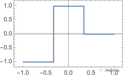
For this task, we’ll need a network that has just one input and one output, like:

为了完成这个任务，我们需要一个只有一个输入和一个输出的网络，像这样：

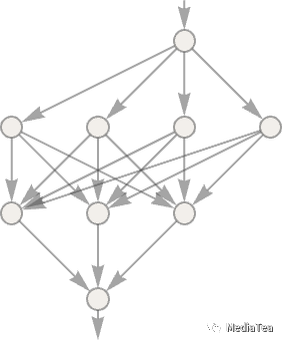
But what weights, etc. should we be using? With every possible set of weights the neural net will compute some function. And, for example, here’s what it does with a few randomly chosen sets of weights:

但是我们应该使用什么样的权重等参数呢？对于每一组可能的权重，神经网络都会计算出某个函数。例如，以下是它对几组随机选择的权重所做的操作：

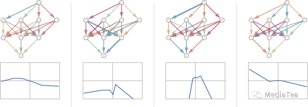
And, yes, we can plainly see that in none of these cases does it get even close to reproducing the function we want. So how do we find weights that will reproduce the function?

是的，我们可以明显看到，在这些情况下，它都没有接近我们想要的函数。那么我们如何找到能复现这个函数的权重呢？

The basic idea is to supply lots of “input → output” examples to “learn from”—and then to try to find weights that will reproduce these examples. Here’s the result of doing that with progressively more examples:

基本的想法是提供大量的“输入 → 输出”的例子来“学习”，然后尝试找到能复现这些例子的权重。以下是用越来越多的例子进行尝试的结果：

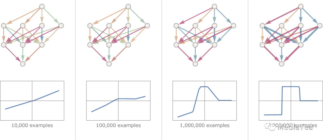
At each stage in this “training” the weights in the network are progressively adjusted—and we see that eventually we get a network that successfully reproduces the function we want. So how do we adjust the weights? The basic idea is at each stage to see “how far away we are” from getting the function we want—and then to update the weights in such a way as to get closer.

在这个“训练”过程的每个阶段，网络中的权重逐渐进行调整，最终我们得到了一个能够成功复现我们所需功能的网络。那么我们如何调整权重呢？基本思路是在每个阶段检查我们离获得期望的函数有多远，并以某种方式更新权重以更接近目标。

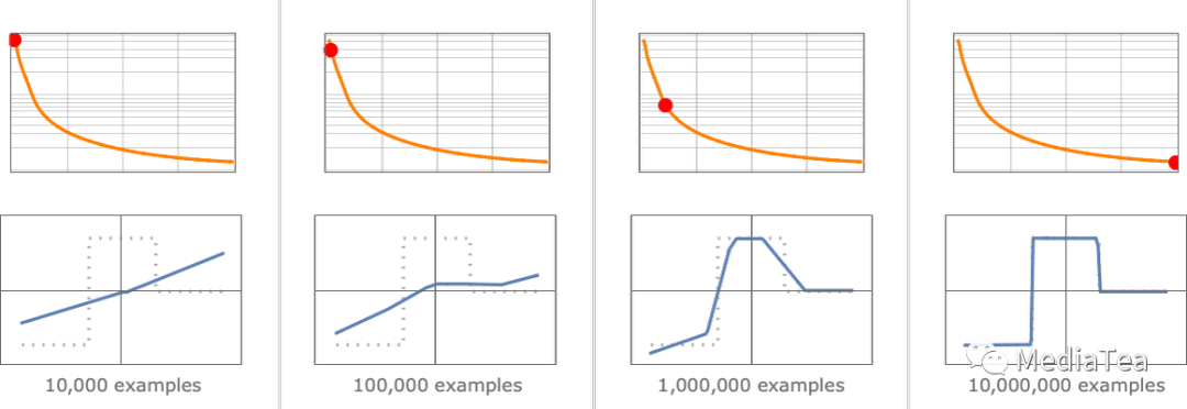
To find out “how far away we are” we compute what’s usually called a “loss function” (or sometimes “cost function”). Here we’re using a simple (L2) loss function that’s just the sum of the squares of the differences between the values we get, and the true values. And what we see is that as our training process progresses, the loss function progressively decreases (following a certain “learning curve” that’s different for different tasks)—until we reach a point where the network (at least to a good approximation) successfully reproduces the function we want:

为了找出“我们有多远”，我们通常会计算一个被称为“损失函数”（或有时叫做“成本函数”）。这里我们使用了一个简单的（L2）损失函数，它只是我们得到的值和真实值之间差的平方和。我们看到的是，随着我们的训练过程的推进，损失函数逐渐减小（遵循不同任务有不同的“学习曲线”）——直到我们达到一个网络（至少在很好的近似程度上）成功复现了我们想要的函数的点：

Alright, so the last essential piece to explain is how the weights are adjusted to reduce the loss function. As we’ve said, the loss function gives us a “distance” between the values we’ve got, and the true values. But the “values we’ve got” are determined at each stage by the current version of neural net—and by the weights in it. But now imagine that the weights are variables—say wi. We want to find out how to adjust the values of these variables to minimize the loss that depends on them.

好的，最后一个需要解释的关键部分是如何调整权重以减小损失函数。如前所述，损失函数给我们提供了我们得到的值与真实值之间的“距离”。但是，“我们得到的值”在每个阶段都是由当前版本的神经网络及其权重决定的。现在假设权重是变量，设为 wi。我们想要找出如何调整这些变量的值以最小化依赖于它们的损失。

For example, imagine (in an incredible simplification of typical neural nets used in practice) that we have just two weights w1 and w2. Then we might have a loss that as a function of w1 and w2 looks like this:

例如，想象一下（在实际应用中对典型神经网络进行极大简化），我们只有两个权重 w1 和 w2。然后，我们可能会有一个损失函数，它作为 w1 和 w2的函数，如下所示：

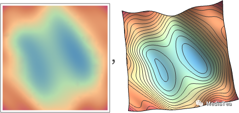
Numerical analysis provides a variety of techniques for finding the minimum in cases like this. But a typical approach is just to progressively follow the path of steepest descent from whatever previous w1, w2 we had:

数值分析提供了各种技术来寻找像这样的情况下的最小值。但是一个典型的方法就是从我们以前的 w1，w2 开始，逐步跟随最陡峭的下降路径：

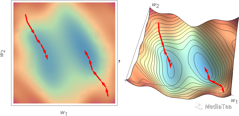
Like water flowing down a mountain, all that’s guaranteed is that this procedure will end up at some local minimum of the surface (“a mountain lake”); it might well not reach the ultimate global minimum.

就像水流沿着山脉流下来，这个过程所能保证的只是它会最终到达表面的某个局部最小值（“山中湖泊”）；但它可能无法达到最终的全局最小值。

It’s not obvious that it would be feasible to find the path of the steepest descent on the “weight landscape”. But calculus comes to the rescue. As we mentioned above, one can always think of a neural net as computing a mathematical function—that depends on its inputs, and its weights. But now consider differentiating with respect to these weights. It turns out that the chain rule of calculus in effect lets us “unravel” the operations done by successive layers in the neural net. And the result is that we can—at least in some local approximation—“invert” the operation of the neural net, and progressively find weights that minimize the loss associated with the output.

找到“权重景观”上最陡峭下降的路径并不明显。但微积分来解救了我们。如我们上面提到的，人们总是可以将神经网络看作计算一个数学函数——它取决于其输入和权重。但现在考虑相对于这些权重的微分。结果证明，微积分的链式法则实际上可以让我们“解开”神经网络连续层所执行的操作。结果是我们可以——至少在一些局部近似中——“反转”神经网络的操作，并逐步找到最小化与输出相关的损失的权重。

The picture above shows the kind of minimization we might need to do in the unrealistically simple case of just 2 weights. But it turns out that even with many more weights (ChatGPT uses 175 billion) it’s still possible to do the minimization, at least to some level of approximation. And in fact the big breakthrough in “deep learning” that occurred around 2011 was associated with the discovery that in some sense it can be easier to do (at least approximate) minimization when there are lots of weights involved than when there are fairly few.

上面的图片展示了我们可能需要在非常简化的情况下，仅针对两个权重进行最小化的情况。但事实证明，即使在有更多权重的情况下（ChatGPT 使用了 1750 亿个权重），仍然可以进行最小化处理，至少可以在一定程度上进行近似。事实上，大约在 2011 年发生的“深度学习”的重大突破与这样一个发现有关：在某种意义上，当涉及到大量权重时，进行（至少是近似的）最小化可能比涉及较少权重时更容易。

In other words—somewhat counterintuitively—it can be easier to solve more complicated problems with neural nets than simpler ones. And the rough reason for this seems to be that when one has a lot of “weight variables” one has a high-dimensional space with “lots of different directions” that can lead one to the minimum—whereas with fewer variables it’s easier to end up getting stuck in a local minimum (“mountain lake”) from which there’s no “direction to get out”.

换句话说，有些违反直觉的是，用神经网络解决更复杂的问题比解决更简单的问题更容易。这似乎主要是因为，当有很多“权重变量”时，人们拥有一个高维空间，其中有“很多不同的方向”可以引导人们找到最小值。而在变量较少的情况下，容易陷入局部最小值（“山间湖泊”），从那里没有“逃脱的方向”。

It’s worth pointing out that in typical cases there are many different collections of weights that will all give neural nets that have pretty much the same performance. And usually in practical neural net training there are lots of random choices made—that lead to “different-but-equivalent solutions”, like these:

值得指出的是，在典型情况下，有许多不同的权重组合，它们都可以使神经网络具有相差无几的性能。通常在实际的神经网络训练中，会进行很多随机选择，这些选择会导致“不同但等效的解决方案”，如下所示：

But each such “different solution” will have at least slightly different behavior. And if we ask, say, for an “extrapolation” outside the region where we gave training examples, we can get dramatically different results:

但是每一个这样的“不同解决方案”都将至少具有稍微不同的行为。如果我们要求在我们给出训练示例的区域之外进行“外推”，我们可能会得到截然不同的结果：

But which of these is “right”? There’s really no way to say. They’re all “consistent with the observed data”. But they all correspond to different “innate” ways to “think about” what to do “outside the box”. And some may seem “more reasonable” to us humans than others.

但是，这些中哪一个是“正确”的呢？实际上没有办法说清楚。它们都是“与观察到的数据一致的”。但是它们都对应了不同的“天生的”方式，来“思考”如何在“框架之外”进行操作。而其中一些可能对我们人类来说，看起来比其他的“更合理”。

“点赞有美意，赞赏是鼓励”