该数据集是从渥太华大学采集的轴承振动信号,这些信号是在时间变化的转速条件下收集的。数据集包含4个不同引擎的每个引擎的12秒信号数据。采样频率为10000

代码主要流程:
-
数据导入与预处理:
- 通过
scipy.io.loadmat()函数从"dataset.mat"文件中加载数据集,其中包含了不同类别的时间序列数据。 - 将不同类别的时间序列数据存储到
df_normal、df_inner、df_roller、df_outer四个数组中。 - 将数据按照类别存储到
data数组中,同时将类别名称存储到label数组中。 - 定义类别标签映射的字典
label_dic。
- 通过
-
数据划分与预测:
- 定义了函数
instancing_data()用于生成训练集和测试集。函数根据给定的train_size和sample_duration参数,将数据划分为训练集和测试集,并对每个实例应用自回归模型进行预测。 - 调用
instancing_data()函数,得到训练集df_train和测试集df_test。 - 从训练集中取出一些样本实例数据,分别命名为
xtb、xth、xtd。 - 使用
statsmodels.tsa.ar_model.AutoReg类创建并拟合自回归模型,对xtb数据进行预测得到xth_pred和xtd_pred。
- 定义了函数
-
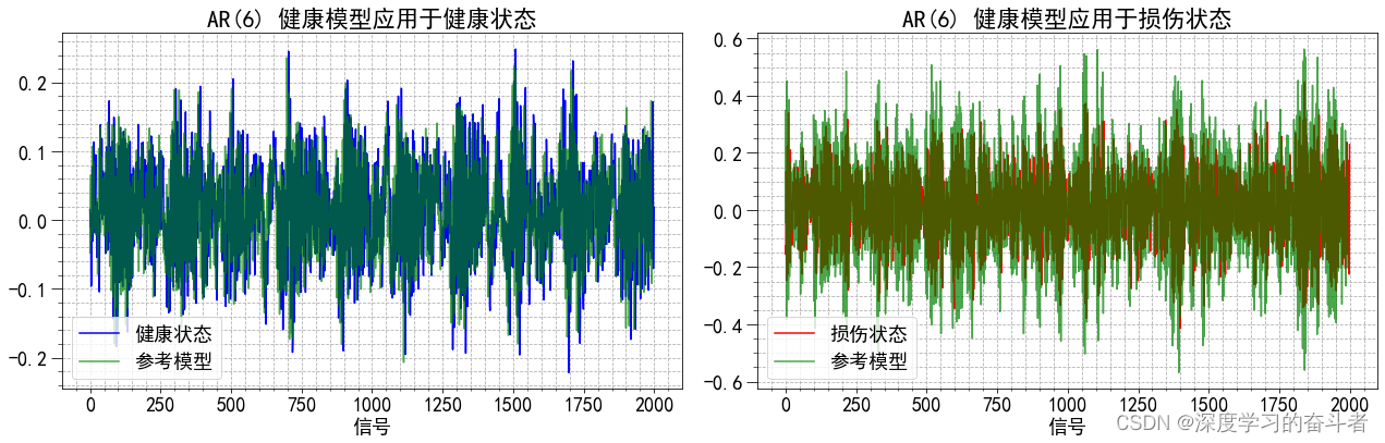
可视化:
- 使用Matplotlib库绘制两个子图,分别展示预测的健康状态和损坏状态与真实值的对比。
-
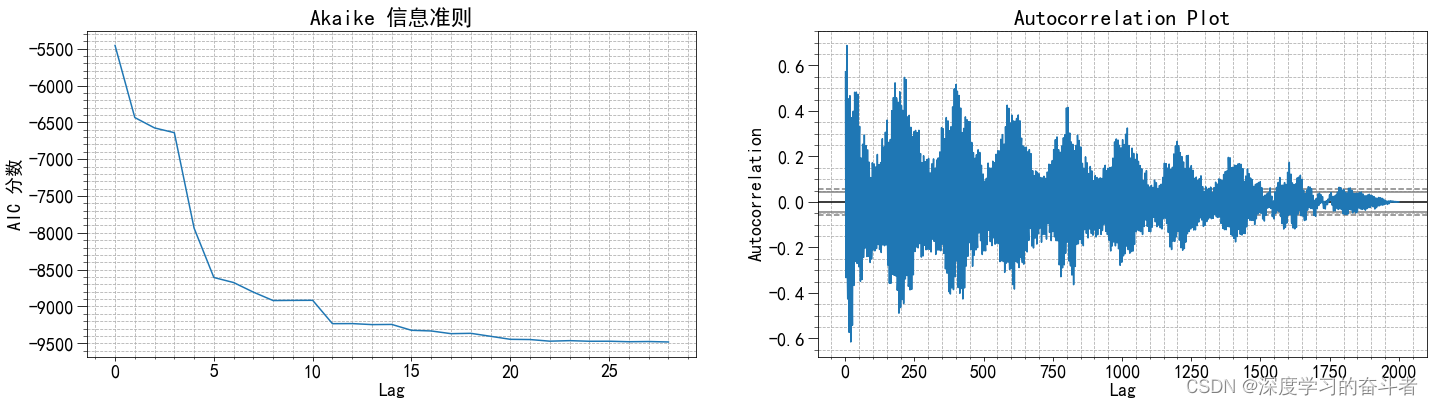
自回归模型评估:
- 创建自回归模型对象,并对样本数据
xt进行不同滞后阶数的拟合,计算AIC值(Akaike information criterion)并绘制AIC值的变化趋势图。 - 绘制样本数据的自相关图。
- 创建自回归模型对象,并对样本数据
-
特征提取:
- 定义了函数
feature_extraction()用于特征提取。该函数对训练集中的每个实例应用自回归模型,并计算特定特征值gamma1和gamma2。 gamma1和gamma2分别用于衡量每个实例的预测残差与整体残差的方差比例和模型参数的方差比例。- 通过特征提取得到了特征数据
df_train_ex。
- 定义了函数
-
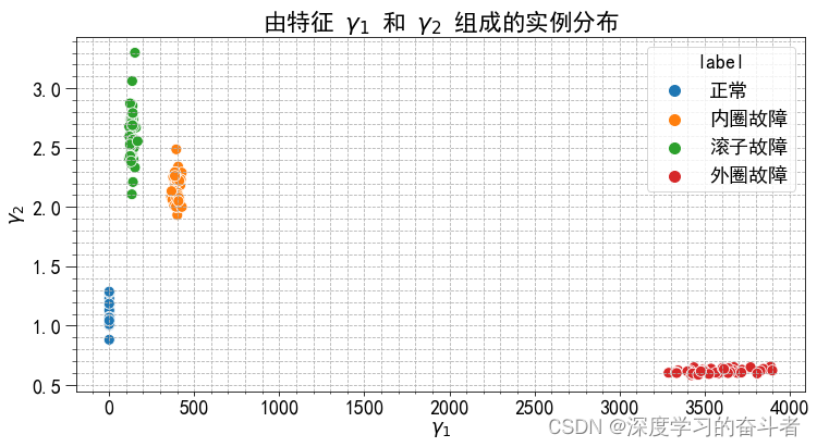
特征可视化:
- 绘制了特征
gamma1和gamma2的散点图,并按照类别进行着色。
- 绘制了特征
-
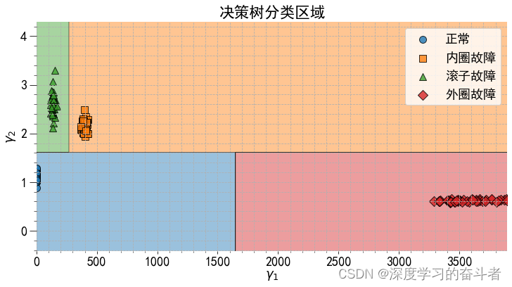
决策树分类:
- 使用
sklearn.tree.DecisionTreeClassifier创建决策树分类器,并对特征数据进行拟合。 - 使用Graphviz库绘制决策树图,并绘制分类区域图。
- 使用
-
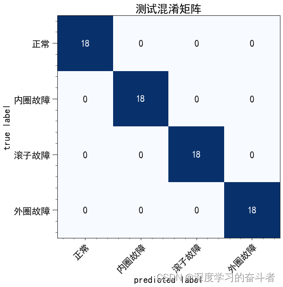
测试集分类:
- 对测试集进行分类预测,并生成混淆矩阵。
-
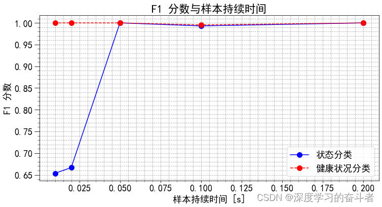
不同样本持续时间下的分类评分:
- 创建决策树分类器,并分别计算不同样本持续时间下的分类评分(F1 Score)。
- 绘制样本持续时间和分类评分之间的关系图。
总体来说,这段代码涉及了时间序列数据的处理、特征提取、模型拟合、分类预测等步骤,并通过可视化展示了各个阶段的结果和评估指标。
完整代码如下:
运行版本要求:
scipy version>=: 1.7.3
numpy version>=: 1.19.2
pandas version>=: 1.2.0
graphviz version>=: 0.16
seaborn version>=: 0.11.1
matplotlib version>=: 3.4.2
python>=3.6.0
import scipy
from scipy import io
import numpy as np
import pandas as pd
import graphviz
import seaborn as sns
import matplotlib.pyplot as plt
plt.rcParams['font.sans-serif']=['simhei'] # 添加中文字体为黑体
plt.rcParams['axes.unicode_minus'] =False
import matplotlib as mpl
from statsmodels.tsa.ar_model import AutoReg
from sklearn import tree
from sklearn.metrics import f1_score
from sklearn.tree import DecisionTreeClassifier as DTC
from mlxtend.plotting import plot_decision_regions, plot_confusion_matrix
from mlxtend.evaluate import confusion_matrix
custom_plot = {'font.serif':'Computer Modern Roman',
'font.size': 18,
'text.usetex': False,
'axes.grid.which': 'both',
'axes.grid': True,
'grid.linestyle': '--',
'xtick.minor.visible':True,
'ytick.minor.visible':True,
'ytick.minor.size':4,
'ytick.major.size':10,
'lines.markersize': 10.0,
}
mpl.rcParams.update(custom_plot)
file = "dataset.mat"
dataset = scipy.io.loadmat(file)
df_normal = dataset["normal"].reshape(-1)
df_inner = dataset["inner"].reshape(-1)
df_roller = dataset["roller"].reshape(-1)
df_outer = dataset["outer"].reshape(-1)
data = [df_normal,df_inner,df_roller,df_outer]
label = ['正常', '内圈故障', '滚子故障', '外圈故障']
label_dic = {0: '正常',
1: '内圈故障',
2: '滚子故障',
3: '外圈故障'}
frequency = 10000
def instancing_data(train_size = 0.7, sample_duration = 0.2):
df_test = pd.DataFrame(columns=('signal', 'label', 'instance'))
df_train = df_test.copy()
for j, arr in enumerate(data):
size = arr.size
samples = sample_duration * frequency
n_instances = size / samples
if n_instances > int(n_instances):
n_instances += 1
samples = int(samples)
n_instances = int(n_instances)
for i in range(n_instances):
signal = arr[0+samples*i:samples*(i+1)]
df_aux = pd.DataFrame({'signal': signal, 'label': j, 'instance': i + n_instances * j})
if i < n_instances * train_size:
df_train = df_train.append(df_aux, ignore_index = True)
else:
df_test = df_test.append(df_aux, ignore_index = True)
return df_train, df_test
df_train, df_test = instancing_data()
xtb = df_train.loc[df_train['instance'] == 0, 'signal'].to_numpy()
xth = df_train.loc[df_train['instance'] == 10, 'signal'].to_numpy()
xtd = df_train.loc[df_train['instance'] == 153, 'signal'].to_numpy()
ar = 6
model = AutoReg(xtb, ar, old_names = False).fit()
params = model.params[1:]
bias = model.params[0]
xth_pred = np.sum([xth[k:xth.size-ar+k] * p for k, p in enumerate(params[::-1])], axis = 0) + bias
xtd_pred = np.sum([xtd[k:xtd.size-ar+k] * p for k, p in enumerate(params[::-1])], axis = 0) + bias
fig, ax = plt.subplots(1, 2, figsize= (18, 6))
ax[0].plot(xth, color = 'b', label = '健康状态')
ax[0].plot(xth_pred, label = '参考模型', color = 'g', alpha = 0.7);
ax[0].set_title(f'AR({ar}) 健康模型应用于健康状态')
ax[1].plot(xtd, color = 'r', label = '损伤状态')
ax[1].plot(xtd_pred, label = '参考模型', color = 'g', alpha = 0.7);
ax[1].set_title(f'AR({ar}) 健康模型应用于损伤状态')
ax[0].legend()
ax[1].legend()
ax[0].set_xlabel('信号')
ax[1].set_xlabel('信号')
fig.tight_layout()
xt = df_train.loc[df_train['instance'] == 0, 'signal']
AIC = []
for i in range(1, 30):
model = AutoReg(xt.to_numpy(), i, old_names = False)
res = model.fit()
AIC.append(res.aic)
fig, ax = plt.subplots(1, 2, figsize=(24, 6))
ax[0].plot(AIC)
ax[0].set_xlabel('Lag')
ax[0].set_ylabel('AIC 分数')
ax[0].set_title('Akaike 信息准则')
pd.plotting.autocorrelation_plot(xt, ax=ax[1])
ax[1].set_title('自相关图');
def feature_extraction(df, xtb, ar = 11):
er_model = AutoReg(xtb.to_numpy(), ar, old_names = False).fit()
instances = df['instance'].unique()
n_instances = instances.size
var_er_pred = np.var(er_model.resid)
var_er_coef = np.var(er_model.params)
gamma1 = []
gamma2 = []
label = []
for i in range(n_instances):
xt = df.loc[df['instance'] == instances[i], 'signal']
ei_model = AutoReg(xt.to_numpy(), ar, old_names = False).fit()
params = er_model.params[1:]
bias = er_model.params[0]
xtp = np.sum([xt[k:xt.size-ar+k] * p for k, p in enumerate(params[::-1])], axis = 0) + bias
var_ei_pred = np.var(xt[ar:]-xtp)
var_ei_coef = np.var(ei_model.params)
gamma1.append(var_ei_pred/var_er_pred)
gamma2.append(var_ei_coef/var_er_coef)
label.append(df.loc[df['instance'] == instances[i], 'label'].iat[0])
df_result = pd.DataFrame({'instance': range(n_instances), 'g1': gamma1, 'g2': gamma2, 'label': label})
return df_result
df_train_ex = feature_extraction(df_train, df_train.loc[df_train['instance'] == 0, 'signal'])
df_aux = df_train_ex.replace({'label': label_dic})
fig, ax = plt.subplots(1, 1, figsize=(12, 6))
ax.set_title('由特征 $\gamma_1$ 和 $\gamma_2$ 组成的实例分布')
sns.scatterplot(data=df_aux, x='g1', y = 'g2', hue='label', ax=ax)
ax.set_xlabel('$\gamma_1$')
ax.set_ylabel('$\gamma_2$');
X_train = df_train_ex[['g1', 'g2']]
y_train = df_train_ex['label']
model = DTC(max_depth=2)
model.fit(X_train.to_numpy(), y_train)
dot_data = tree.export_graphviz(model, out_file=None,
feature_names= ['Gamma 1', 'Gamma 2'],
class_names=label,
label='root',
filled=True)
# Draw graph
graph = graphviz.Source(dot_data, format="png")
graph
fig, ax = plt.subplots(1, 1, figsize=(12, 6))
ax.set_title('决策树分类区域')
plot_decision_regions(X_train.to_numpy(), y_train.to_numpy(),
clf=model, markers = ('o', 's', '^', 'D'),
ax=ax,
)
ax.set_xlabel('$\gamma_1$')
ax.set_ylabel('$\gamma_2$')
L=ax.legend()
for i in range(4):
L.get_texts()[i].set_text(label[i])
df_test_ex = feature_extraction(df_test, df_train.loc[df_train['instance'] == 0, 'signal'])
X_test = df_test_ex[['g1', 'g2']].to_numpy()
y_test = df_test_ex['label']
y_pred = model.predict(X_test)
mpl.rcParams.update({'axes.grid': False})
cm = confusion_matrix(y_test, y_pred)
fig, ax = plot_confusion_matrix(cm, figsize=(8, 8), class_names=label)
ax.set_title('测试混淆矩阵')
model = DTC(max_depth=2)
sample_durations = [0.2, 0.1, 0.05, 0.02, 0.01]
class_scores = []
binary_scores = []
for sd in sample_durations:
df_train, df_test = instancing_data(sample_duration = sd)
df_train_ex = feature_extraction(df_train, df_train.loc[df_train['instance'] == 0, 'signal'])
X_train = df_train_ex[['g1', 'g2']].to_numpy()
y_train = df_train_ex['label']
df_test_ex = feature_extraction(df_test, df_train.loc[df_train['instance'] == 0, 'signal'])
X_test = df_test_ex[['g1', 'g2']].to_numpy()
y_test = df_test_ex['label']
model.fit(X_train, y_train)
y_pred = model.predict(X_test)
y_test_bin = y_test.copy()
y_pred_bin = y_pred.copy()
y_test_bin[y_test_bin > 0] = 1
y_pred_bin[y_pred_bin > 0] = 1
f1 = f1_score(y_test, y_pred, average = 'macro')
f1_bin = f1_score(y_test_bin, y_pred_bin)
class_scores.append(f1)
binary_scores.append(f1_bin)
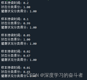
print(f'样本持续时间: {sd}\n状态分类得分: {f1:.2f}\n健康状况分类得分: {f1_bin:.2f}\n')
mpl.rcParams.update({'axes.grid': True})
fig, ax = plt.subplots(1, 1, figsize=(12, 6))
ax.plot(sample_durations, class_scores, ls = '-', marker = 'o', color='b', label = '状态分类')
ax.plot(sample_durations, binary_scores, ls = '--', marker = 'o', color='r', label = '健康状况分类')
ax.set_xlabel('样本持续时间 [s]')
ax.set_ylabel('F1 分数')
ax.set_title('F1 分数与样本持续时间')
ax.legend();
若对数据集和代码放在一起的压缩包感兴趣可以关注下面最后一行:
import scipy
from scipy import io
import numpy as np
import pandas as pd

import graphviz


import seaborn as sns
import matplotlib.pyplot as plt
plt.rcParams['font.sans-serif']=['simhei'] # 添加中文字体为黑体
plt.rcParams['axes.unicode_minus'] =False
import matplotlib as mpl

from statsmodels.tsa.ar_model import AutoReg
from sklearn import tree
from sklearn.metrics import f1_score
from sklearn.tree import DecisionTreeClassifier as DTC

from mlxtend.plotting import plot_decision_regions, plot_confusion_matrix
from mlxtend.evaluate import confusion_matrix
#代码和数据集放在一起的压缩包:https://mbd.pub/o/bread/ZJyUlZxp