Reinforcement Learning with Code

This note records how the author begin to learn RL. Both theoretical understanding and code practice are presented. Many material are referenced such as ZhaoShiyu’s Mathematical Foundation of Reinforcement Learning, .

Chapter 8. Value Funtion Approximation

​ As so far in this note, state and action values are represented in tabular fashion. There are two problems that first although tabular representation is intuitive, it would encounter some problems when the state action space is large. Second since the value of a state is updated only if it is visited, the values of unvisited states cannot be estimated.

​ We can sovle the problems using a parameterized function $\hat{v}(s,w)$ to approximate the value funtion, where $w\in {\mathbb{R}}^m$ is the parameter vector. On the one hand, we only need to store the parameter $w$ instead of all states $s$, which is much smaller. On the other hand, when a state $s$ is visited, the parameter $w$ is updated so that the values of some other unvisited states can also be estimated.

​ We usually use neural network to approximate the value function. This problem basically is a regression problem. We can find the optimal parameter $w$ by minimize some objective funtions, which we will introduce next.

8.1 State value: MC/TD learning with function approximation

​ Let $v_{\pi }(s)$ and $\hat{v}(s,w)$ be the true value and approximated state value of $s\in \mathcal{S}$. The objective funtion considered in value function approximation is usually
$$J(w)=\mathbb{E}\left[\right(v_{\pi }(S)-\hat{v}(S,w){)}^2]$$
which is also called mean square error in deep learning field. Where $S,S^{\prime }$ denote random variable of state $s$.

​ Next, we discuss the distribution of random variable $S$. We often use the stationary distribution, which describeds the long-run behavior of a Markov process. Let { d π ( s ) } s ∈ S \textcolor{blue}{\{d_\pi(s)\}_{s\in\mathcal{S}}} {dπ​(s)}s∈S​ donte the stationary distribution of random variable $S$. By definition, $d_{\pi }(s)\ge 0$ and ${\sum }_{s\in \mathcal{S}}{d}_{\pi }(s)=1$. Hence, the objective funciton can be rewritten as
$$J(w)=\sum _{s\in \mathcal{S}}{d}_{\pi }(s)[v_{\pi }(s)-\hat{v}(s,w){]}^2$$
This objective function is a weighted squared error. How to compute the stationary distribution of random variable $S$? We often use the equation
$$d_{\pi }^T=d_{\pi }^T{P}_{\pi }$$
As a result, $d_{\pi }$ is the left eigenvector of $P_{\pi }$ associated with the eigenvalue of $1$. The proof is omitted.

Recall the spirit of gradient descent (GD). We can use it to minimize the objective function as
$$\begin{array}{rl}{w}_{k+1}& =w_k-{\alpha }_k{\nabla }_w\mathbb{E}[(v_{\pi }(S)-\hat{v}(S,w){)}^2]\\ & =w_k-{\alpha }_k\mathbb{E}[{\nabla }_w(v_{\pi }(S)-\hat{v}(S,w){)}^2]\\ & =w_k-2{\alpha }_k\mathbb{E}[(v_{\pi }(S)-\hat{v}(S,w)){\nabla }_w(-\hat{v}(S,w))]\\ & =w_k+2{\alpha }_k\mathbb{E}[v_{\pi }(S)-\hat{v}(S,w){\nabla }_w\hat{v}(S,w)]\end{array}$$
where without loss of generality the cofficient 2 before ${\alpha }_k$ can be dropped. By the spirit of stochastic gradient descent (SGD), we can remove the expectation operation to obtain
$$w_{t+1}=w_t+a_t(v_{\pi }(s_t)-\hat{v}(s_t,w_t)){\nabla }_w\hat{v}(s_t,w_t)$$
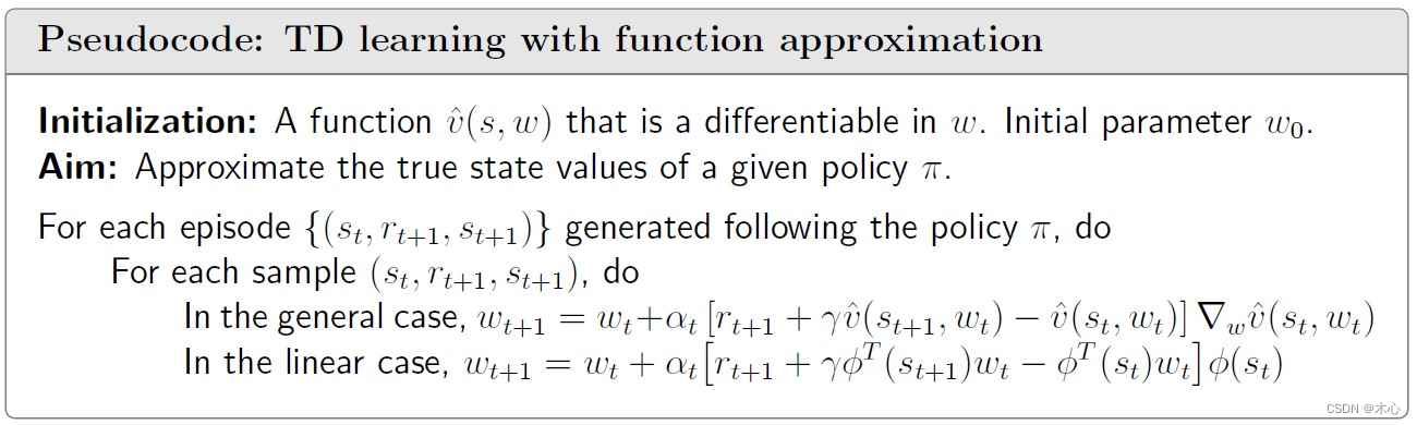
However this equation can’t be implemented. Because it requires the true state value $v_{\pi }$, which is the unknown to be esitmated. Hence, we can use the idea of Monte Carlo or TD learning to estimate it.

​ By Monte Carlo learning spirit, we can use the $g_t$ to denote the discounted return that
$$g_t=r_{t+1}+\gamma r_{t+2}+{\gamma }^2{r}_{t+3}+\cdots$$
Then, $g_t$ can be used as an approximation of $v_{\pi }(s)$. The algorithm becomes
$$w_{t+1}=w_t+a_t(g_t-\hat{v}(s_t,w_t)){\nabla }_w\hat{v}(s_t,w_t)$$
​ By TD learning spirit, we can use the $r_{t+1}+\gamma \hat{v}(s_{t+1},w_t)$ as the approximation of $v_{\pi }(s)$. The algorithm becomes
$$w_{t+1}=w_t+a_t(r_{t+1}+\gamma \hat{v}(s_{t+1},w)-\hat{v}(s_t,w_t)){\nabla }_w\hat{v}(s_t,w_t)$$
Pesudocode:

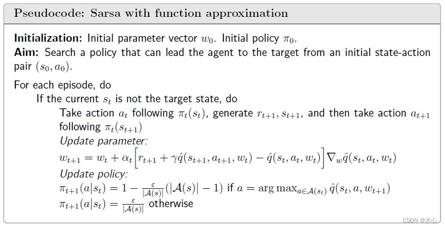
8.2 Action value: Sarsa with funtion approximation

​ To seach for optimal policies, we need to estimate action values. This section introduces how to estimate action values using Sarsa in the presence of value function approximation.

​ The action value $q_{\pi }(s,a)$ is described by a function $\hat{q}(s,a,w)$ parameterized by $w$. The objective funtion considered in action value approximation is usually selected as
$$J(w)=\mathbb{E}[(q_{\pi }(S,A)-\hat{q}(S,A,w){)}^2]$$
Use the stochasitic gradient descent to minimize the objective function

$$\begin{array}{rl}{w}_{k+1}& =w_k-{\alpha }_k{\nabla }_w\mathbb{E}[(q_{\pi }(S,A)-\hat{q}(S,A,w){)}^2]\\ & =w_k+2a_k\mathbb{E}[q_{\pi }(S,A)-\hat{q}(S,A,w)]{\nabla }_w\hat{q}(S,A,w)\\ & =w_k+{\alpha }_k(q_{\pi }(s,a)-\hat{q}(s,a,w)){\nabla }_w\hat{q}(s,a,w)\end{array}$$

where without loss of generality the cofficient 2 before ${\alpha }_k$ can be dropped.

​ By Sarsa spirit, we use the $r+\gamma \hat{q}(s^{\prime },a^{\prime },w)$ to approximate ture action value $q_{\pi }(s,a)$. Hence we have
$$w_{k+1}=w_k+{\alpha }_k(r+\gamma \hat{q}(s^{\prime },a^{\prime },w)-\hat{q}(s,a,w)){\nabla }_w\hat{q}(s,a,w)$$
The sampled data $(s,a,r_k,s_k^{\prime },a_k^{\prime })$ is changed to $(s_t,a_t,r_{t+1},s_{t+1},a_{t+1})$. Hence
$$w_{t+1}=w_t+{\alpha }_t[r_{t+1}+\gamma \hat{q}(s_{t+1},a_{t+1},w_t)-\hat{q}(s_t,a_t,w_t)]{\nabla }_w\hat{q}(s_t,a_t,w_t)$$
Pseudocode:

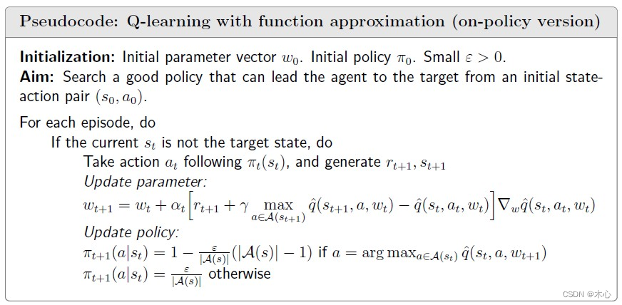
8.3 Optimal action value: Q-learning with function approximation

​ Similar to Sarsa, tabular Q-learning can also be extended to the case of value function approximation.

By the spirit of Q-learning, the update rule is

$$w_{t+1}=w_t+{\alpha }_t[r_{t+1}+\gamma \underset{a\in \mathcal{A}(s_{t+1})}{\max }\hat{q}(s_{t+1},a,w_t)-\hat{q}(s_t,a_t,w_t)]{\nabla }_w\hat{q}(s_t,a_t,w_t)$$
which is the same as Sarsa expect that $\hat{q}(s_{t+1},a_{t+1},w_t)$ is replaced by ${\max }_{a\in \mathcal{A}(s_{t+1})}\hat{q}(s_{t+1},a,w_t)$.

Pseudocode:

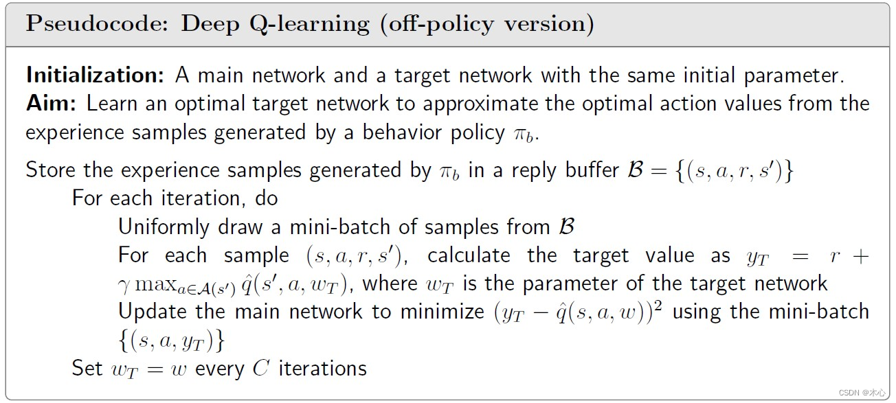
8.4 Deep Q-learning (DQN)

​ We can introduce deep neural networks into Q-learning to obtain deep Q-learning or deep Q-network (DQN).

Mathematically, deep Q-learning aims to minimize the objective funtion
$$J(w)=\mathbb{E}\left[\right(R+\gamma \underset{a\in \mathcal{A}(S^{\prime })}{\max }\hat{q}(S^{\prime },a,w)-\hat{q}(S,A,w){)}^2]$$
where $(S,A,R,S^{\prime })$ are random variables representing a state, an action taken at that state, the immediate reward, and the next state. This objective funtion can be viewed as the Bellman opitmality error. That is because
$$q(s,a)=\mathbb{E}[R_{t+1}+\gamma \underset{a\in \mathcal{A}(S_{t+1})}{\max }q(S_{t+1},a)|S_t=s,A_t=a]$$
is the Bellman optimality equation in terms of action value.

​ Then we can use the stochastic gradient to minimize the objective funtion. However, it is noted that the parameter $w$ not only apperas in $\hat{q}(S,A,w)$ but also in $y\triangleq R+\gamma {\max }_{a\in \mathcal{A}(S^{\prime })}\hat{q}(S^{\prime },a,w)$. For the sake of simplicity, we can assume that $w$ in $y$ is fixed (at least for a while) when we calculate the gradient. To do that, we can introduce two networks. One is a *main networ*k representing $\hat{q}(s,a,w)$ and the other is a target network $\hat{q}(s,a,w_T)$. The objective function in this case degenerates to
$$J(w)=\mathbb{E}\left[\right(R+\gamma \underset{a\in \mathcal{A}(S^{\prime })}{\max }\hat{q}(S^{\prime },a,w_T)-\hat{q}(S,A,w){)}^2]$$
where $w_T$ is the target network parameter and $w$ is the main network parameter. When $w_T$ is fixed, the gradient of $J(w)$ is
$${\nabla }_{w}J=-2\ast \mathbb{E}\left[\right(R+\gamma \underset{a\in \mathcal{A}(S^{\prime })}{\max }\hat{q}(S^{\prime },a,w_T)-\hat{q}(S^{\prime },A,w)){\nabla }_w\hat{q}(S,A,w)]$$
There are two techniques should be noticed.

​ When the target network is fixed, using stochastic gradient descent (SGD) we can obtain
$$w_{t+1}=w_t+{\alpha }_t[r_{t+1}+\gamma \underset{a\in \mathcal{A}(s_{t+1})}{\max }\hat{q}(s_{t+1},a,w_T)-\hat{q}(s_t,a_t,w)]{\nabla }_w\hat{q}(s_t,a_t,w)$$
​ One technique is experience replay. This is, after we have collected some experience samples, we don’t use these samples in the order they were collected. Instead, we store them in a data set, called replay buffer, and draw a batch of samples randomly to train the neureal network. In particular, let $(s,a,r,s^{\prime })$ be an experience sample and $\mathcal{B}\triangleq \{(s,a,r,s^{\prime })\}$ be the replay buffer. Every time we train the neural network, we can draw a mini-batch of random samples from the reply buffer. The draw of samples, or called experience replay, should follow a uniform distribution.

​ Another technique is use two networks. A main network parameterized by $w$, and a target network parameterized by $w_T$. The two network parameters are set to be the same initially. The target output is $y_T\triangleq r+\gamma {\max }_{a\in \mathcal{A}(s^{\prime })}\hat{q}(s^{\prime },a,w_T)$. Then, we directly minimize the TD error or called loss function $(y-\hat{q}(s,a,w,){)}^2$ over the mini-batch $\{(s,a,y_T)\}$ instead of a single sample to improve efficiency and stability.

​ The parameter of the main network is updated in every interation. By contrast, the target network is set to be the same as the main network every a certain number of iterations to meet the assumption that $w_T$ is fixed when calculating the gradient.

Pseudocode:

---

Reference

赵世钰老师的课程