本文参考于 https://eigen.tuxfamily.org/dox/group__TopicLinearAlgebraDecompositions.html
很多场合我们需要去计算矩阵的特征值与特征向量,但是Eigen中有好几个计算特征值与特征向量的方法,这些方法到底该选哪个呢?这篇文章就带着大家来分析一下。
1 计算特征值与特征向量的方法有如下几种
- BDCSVD
- JacobiSVD
- SelfAdjointEigenSolver
- ComplexEigenSolver
- EigenSolver
- GeneralizedSelfAdjointEigenSolver
2 每个方法的说明
2.1 BDCSVD
功能为:Bidiagonal Divide and Conquer SVD,双对角线分治SVD
类的原型为
template<typename MatrixType_, int Options_>
class Eigen::BDCSVD< MatrixType_, Options_ >
模板参数 MatrixType_: 我们正在计算 SVD 分解的矩阵的类型
模板参数 Options_ : 此可选参数允许指定计算U和V的选项. 可选参数为ComputeThinU,ComputeThinV,ComputeFullU,ComputeFullV。无法同时请求 U 或 V 的精简版和完整版。默认情况下,不计算酉。
此类首先使用类上双对角化将输入矩阵简化为双对角线形式,然后执行分而治之对角化。小块使用类 JacobiSVD 对角化。您可以使用 setSwitchSize() 方法控制切换大小,默认值为 16。因此,对于小矩阵(<16),最好直接使用JacobiSVD。对于较大的,强烈建议使用BDCSVD,并且可以快几个数量级。
画重点,16维以下的矩阵,进行SVD分解,直接使用JacobiSVD,大于等于16维的矩阵,强烈建议使用BDCSVD。
2.2 JacobiSVD
功能为:Two-sided Jacobi SVD decomposition of a rectangular matrix, 长方形矩阵的双侧 Jacobi SVD 分解。
模板参数 MatrixType_:我们正在计算 SVD 分解的矩阵的类型
模板参数 Options_ :此可选参数允许指定将在内部用于非平方矩阵的 R-SVD 步骤的 QR 分解类型。此外,它还允许人们指定是计算薄酉还是全酉U和V。请参阅下面对可能值的讨论
SVD 分解包括将任何 n×p 矩阵 A 分解为乘积 A=USV∗
其中 U 是 n×n ,V 是 p×p ,S 是 n×p 实正矩阵,在其主对角线之外为零;
S 的对角线条目称为 A 的奇异值,U 和 V 的列分别称为 A 的左奇异向量和右奇异向量。
奇异值始终按降序排序。
默认情况下,此 JacobiSVD 分解仅计算奇异值。如果你想要U或V,你需要明确地要求它们。
您可以要求仅计算薄 U 或 V,这意味着以下内容。在矩形 n×p 矩阵的情况下,让 m 是 n 和 p 中的较小值,只有 m 个奇异向量;U 和 V 的其余列与实际的奇异向量不对应。要求细 U 或 V 意味着只要求形成它们的 m 第一列。所以 U 是一个 n×m 矩阵,V 是一个 p×m 矩阵。请注意,瘦 U 和 V 是求解(最小二乘法)所需要的全部内容。
这个 JacobiSVD 类是双侧 JacobiR-SVD 分解,确保了最佳的可靠性和准确性。缺点是对于大的方阵,它比双对角化 SVD 算法慢; 但是它的复杂度仍然是 O (n^2 * p) ,其中 n 是较小的维数,p 是较大的维数,这意味着它的复杂度仍然与更快的双对角化 R-SVD 算法相同。特别地,像任何 R-SVD 一样,它利用了非平方性,因为它的复杂性只在更大的维数上是线性的。如果输入矩阵有 inf 或 nan 系数,计算结果是未定义的,但计算保证在有限(合理)时间内终止。
画重点,16维以下的矩阵,进行SVD分解,直接使用JacobiSVD。
MatrixXf m = MatrixXf::Random(3,2);
cout << "Here is the matrix m:" << endl << m << endl;
JacobiSVD<MatrixXf, ComputeThinU | ComputeThinV> svd(m);
cout << "Its singular values are:" << endl << svd.singularValues() << endl;
cout << "Its left singular vectors are the columns of the thin U matrix:" << endl << svd.matrixU() << endl;
cout << "Its right singular vectors are the columns of the thin V matrix:" << endl << svd.matrixV() << endl;
Vector3f rhs(1, 0, 0);
cout << "Now consider this rhs vector:" << endl << rhs << endl;
cout << "A least-squares solution of m*x = rhs is:" << endl << svd.solve(rhs) << endl;

---

Here is the matrix m:
  0.68  0.597
-0.211  0.823
 0.566 -0.605
Its singular values are:
 1.19
0.899
Its left singular vectors are the columns of the thin U matrix:
  0.388   0.866
  0.712 -0.0634
 -0.586   0.496
Its right singular vectors are the columns of the thin V matrix:
-0.183  0.983
 0.983  0.183
Now consider this rhs vector:
1
0
0
A least-squares solution of m*x = rhs is:
0.888
0.496
2.3 SelfAdjointEigenSolver
功能为:Computes eigenvalues and eigenvectors of selfadjoint matrices. 计算自伴矩阵的特征值与特征矢量。
这是在特征值模块中定义的。
#include <Eigen/Eigenvalues>
首先要考虑一下什么是自伴矩阵。
对于实矩阵,自伴矩阵就是对称矩阵。 对于复数矩阵,自伴是厄米特矩阵的同义词。
更一般地说,矩阵 A 是自伴的,当且仅当它等于它的伴随 A * 。
这个类计算自伴矩阵的特征值与特征矢量。这些是标量 λ 和向量 v,使得 Av = λv。自伴矩阵的特征值总是实的。如果 D 是特征值在对角线上的对角矩阵,V 是以特征向量为列的矩阵,则 A = VDV-1。这就是所谓的特征分解。
对于自伴矩阵,V 是酉矩阵,意味着它的逆等于它的伴随矩阵,V-1 = V*。如果 A 是实的,那么 V 也是实的,因此是正交的,这意味着它的逆等于它的转置,V-1 = VT。算法利用了矩阵是自伴的这一事实,使它比在 EigenSolver 和 ComplexEigenSolver 中实现的通用特征值算法更快、更准确。
调用 computer ()函数来计算给定矩阵的特征矢量。或者,你可以使用 selfAdjointeigenSolver (const matrixType & ,int)构造函数在构造时计算特征矢量。一旦特征值和特征向量被计算出来,它们就可以用 eigenvalues() eigenvectors()函数来检索。
画重点,SelfAdjointEigenSolver是计算实对称矩阵的特征值与特征向量的
SelfAdjointEigenSolver<Matrix4f> es;
Matrix4f X = Matrix4f::Random(4,4);
Matrix4f A = X + X.transpose();
es.compute(A);
cout << "The eigenvalues of A are: " << es.eigenvalues().transpose() << endl;
es.compute(A + Matrix4f::Identity(4,4)); // re-use es to compute eigenvalues of A+I
cout << "The eigenvalues of A+I are: " << es.eigenvalues().transpose() << endl;

The eigenvalues of A are:  -1.58 -0.473   1.32   2.46
The eigenvalues of A+I are: -0.581  0.527   2.32   3.46
MatrixXd X = MatrixXd::Random(5,5);
MatrixXd A = X + X.transpose();
cout << "Here is a random symmetric 5x5 matrix, A:" << endl << A << endl << endl;

SelfAdjointEigenSolver<MatrixXd> es(A);
cout << "The eigenvalues of A are:" << endl << es.eigenvalues() << endl;
cout << "The matrix of eigenvectors, V, is:" << endl << es.eigenvectors() << endl << endl;

double lambda = es.eigenvalues()[0];
cout << "Consider the first eigenvalue, lambda = " << lambda << endl;
VectorXd v = es.eigenvectors().col(0);
cout << "If v is the corresponding eigenvector, then lambda * v = " << endl << lambda * v << endl;
cout << "... and A * v = " << endl << A * v << endl << endl;

MatrixXd D = es.eigenvalues().asDiagonal();
MatrixXd V = es.eigenvectors();
cout << "Finally, V * D * V^(-1) = " << endl << V * D * V.inverse() << endl;

---

Here is a random symmetric 5x5 matrix, A:
  1.36 -0.816  0.521   1.43 -0.144
-0.816 -0.659  0.794 -0.173 -0.406
 0.521  0.794 -0.541  0.461  0.179
  1.43 -0.173  0.461  -1.43  0.822
-0.144 -0.406  0.179  0.822  -1.37

The eigenvalues of A are:
 -2.65
 -1.77
-0.745
 0.227
  2.29
The matrix of eigenvectors, V, is:
 -0.326 -0.0984   0.347 -0.0109   0.874
 -0.207  -0.642   0.228   0.662  -0.232
 0.0495   0.629  -0.164    0.74   0.164
  0.721  -0.397  -0.402   0.115   0.385
 -0.573  -0.156  -0.799 -0.0256  0.0858

Consider the first eigenvalue, lambda = -2.65
If v is the corresponding eigenvector, then lambda * v =
 0.865
  0.55
-0.131
 -1.91
  1.52
... and A * v =
 0.865
  0.55
-0.131
 -1.91
  1.52

Finally, V * D * V^(-1) =
  1.36 -0.816  0.521   1.43 -0.144
-0.816 -0.659  0.794 -0.173 -0.406
 0.521  0.794 -0.541  0.461  0.179
  1.43 -0.173  0.461  -1.43  0.822
-0.144 -0.406  0.179  0.822  -1.37
2.4 ComplexEigenSolver
功能为:Computes eigenvalues and eigenvectors of general complex matrices. 计算一般复数矩阵的特征值与特征向量,这在特征值模块中定义。
#include <Eigen/Eigenvalues>
画重点,ComplexEigenSolver是计算复数矩阵的特征值与特征向量
MatrixXcf A = MatrixXcf::Random(4,4);
cout << "Here is a random 4x4 matrix, A:" << endl << A << endl << endl;

ComplexEigenSolver<MatrixXcf> ces;
ces.compute(A);
cout << "The eigenvalues of A are:" << endl << ces.eigenvalues() << endl;
cout << "The matrix of eigenvectors, V, is:" << endl << ces.eigenvectors() << endl << endl;

complex<float> lambda = ces.eigenvalues()[0];
cout << "Consider the first eigenvalue, lambda = " << lambda << endl;
VectorXcf v = ces.eigenvectors().col(0);
cout << "If v is the corresponding eigenvector, then lambda * v = " << endl << lambda * v << endl;
cout << "... and A * v = " << endl << A * v << endl << endl;

cout << "Finally, V * D * V^(-1) = " << endl
     << ces.eigenvectors() * ces.eigenvalues().asDiagonal() * ces.eigenvectors().inverse() << endl;


Here is a random 4x4 matrix, A:
  (-0.211,0.68)  (0.108,-0.444)   (0.435,0.271) (-0.198,-0.687)
  (0.597,0.566) (0.258,-0.0452)  (0.214,-0.717)  (-0.782,-0.74)
 (-0.605,0.823)  (0.0268,-0.27) (-0.514,-0.967)  (-0.563,0.998)
  (0.536,-0.33)   (0.832,0.904)  (0.608,-0.726)  (0.678,0.0259)

The eigenvalues of A are:
 (0.137,0.505)
 (-0.758,1.22)
 (1.52,-0.402)
(-0.691,-1.63)
The matrix of eigenvectors, V, is:
  (-0.246,-0.106)     (0.418,0.263)   (0.0417,-0.296)    (-0.122,0.271)
  (-0.205,-0.629)    (0.466,-0.457)    (0.244,-0.456)      (0.247,0.23)
 (-0.432,-0.0359) (-0.0651,-0.0146)    (-0.191,0.334)   (0.859,-0.0877)
    (-0.301,0.46)    (-0.41,-0.397)     (0.623,0.328)    (-0.116,0.195)

Consider the first eigenvalue, lambda = (0.137,0.505)
If v is the corresponding eigenvector, then lambda * v =
 (0.0197,-0.139)
    (0.29,-0.19)
(-0.0412,-0.223)
(-0.274,-0.0891)
... and A * v =
 (0.0197,-0.139)
    (0.29,-0.19)
(-0.0412,-0.223)
(-0.274,-0.0891)

Finally, V * D * V^(-1) =
  (-0.211,0.68)  (0.108,-0.444)   (0.435,0.271) (-0.198,-0.687)
  (0.597,0.566) (0.258,-0.0452)  (0.214,-0.717)  (-0.782,-0.74)
 (-0.605,0.823)  (0.0268,-0.27) (-0.514,-0.967)  (-0.563,0.998)
  (0.536,-0.33)   (0.832,0.904)  (0.608,-0.726)  (0.678,0.0259)
2.5 EigenSolver
功能为:Computes eigenvalues and eigenvectors of general matrices. 计算一般矩阵的特征值与特征向量,这在特征值模块中定义。
#include <Eigen/Eigenvalues>
矩阵 a 的特征矢量是标量 λ 和向量 v,使得 Av = λv。
如果 D 是特征值在对角线上的对角矩阵,V 是以特征向量为列的矩阵,则 AV = VD。矩阵 V 几乎总是可逆的,在这种情况下,我们有 A = VDV-1。这就是所谓的特征分解。
矩阵的特征矢量可能很复杂,即使矩阵是真实的。然而,我们可以选择实矩阵 V 和 D 满足 AV = VD,就像特征分解一样,如果矩阵 D 不需要是对角线,但是如果它允许在对角线上有块[ u-vvu ](其中 u 和 v 是实数)。这些块对应于复特征值对 u ± iv。我们称这种特征分解的变体为伪特征分解。
调用 computer ()函数来计算给定矩阵的特征矢量。或者,你也可以使用 eigenSolver (const Matrix Type & ,bool)构造函数来计算构造时的特征矢量。一旦特征值和特征向量被计算出来,它们就可以用eigenvalues() 和 eigenvectors()函数来获取。pseudoEigenvalueMatrix() and pseudoEigenvectors() 方法允许构造伪特征分解。
画重点,EigenSolver是一般矩阵(非对称矩阵,复数矩阵)的特征值与特征向量
MatrixXd A = MatrixXd::Random(6,6);
cout << "Here is a random 6x6 matrix, A:" << endl << A << endl << endl;

EigenSolver<MatrixXd> es(A);
cout << "The eigenvalues of A are:" << endl << es.eigenvalues() << endl;
cout << "The matrix of eigenvectors, V, is:" << endl << es.eigenvectors() << endl << endl;

complex<double> lambda = es.eigenvalues()[0];
cout << "Consider the first eigenvalue, lambda = " << lambda << endl;
VectorXcd v = es.eigenvectors().col(0);
cout << "If v is the corresponding eigenvector, then lambda * v = " << endl << lambda * v << endl;
cout << "... and A * v = " << endl << A.cast<complex<double> >() * v << endl << endl;

MatrixXcd D = es.eigenvalues().asDiagonal();
MatrixXcd V = es.eigenvectors();
cout << "Finally, V * D * V^(-1) = " << endl << V * D * V.inverse() << endl;


Here is a random 6x6 matrix, A:
   0.68   -0.33   -0.27  -0.717  -0.687  0.0259
 -0.211   0.536  0.0268   0.214  -0.198   0.678
  0.566  -0.444   0.904  -0.967   -0.74   0.225
  0.597   0.108   0.832  -0.514  -0.782  -0.408
  0.823 -0.0452   0.271  -0.726   0.998   0.275
 -0.605   0.258   0.435   0.608  -0.563  0.0486

The eigenvalues of A are:
  (0.049,1.06)
 (0.049,-1.06)
     (0.967,0)
     (0.353,0)
 (0.618,0.129)
(0.618,-0.129)
The matrix of eigenvectors, V, is:
 (-0.292,-0.454)   (-0.292,0.454)      (-0.0607,0)       (-0.733,0)    (0.59,-0.121)     (0.59,0.121)
  (0.134,-0.104)    (0.134,0.104)       (-0.799,0)        (0.136,0)    (0.334,0.368)   (0.334,-0.368)
  (-0.422,-0.18)    (-0.422,0.18)        (0.192,0)       (0.0563,0)  (-0.335,-0.143)   (-0.335,0.143)
 (-0.589,0.0274) (-0.589,-0.0274)      (-0.0788,0)       (-0.627,0)   (0.322,-0.155)    (0.322,0.155)
  (-0.248,0.132)  (-0.248,-0.132)        (0.401,0)        (0.218,0) (-0.335,-0.0761)  (-0.335,0.0761)
    (0.105,0.18)    (0.105,-0.18)       (-0.392,0)     (-0.00564,0)  (-0.0324,0.103) (-0.0324,-0.103)

Consider the first eigenvalue, lambda = (0.049,1.06)
If v is the corresponding eigenvector, then lambda * v =
  (0.466,-0.331)
   (0.117,0.137)
   (0.17,-0.456)
(-0.0578,-0.622)
 (-0.152,-0.256)
   (-0.186,0.12)
... and A * v =
  (0.466,-0.331)
   (0.117,0.137)
   (0.17,-0.456)
(-0.0578,-0.622)
 (-0.152,-0.256)
   (-0.186,0.12)

Finally, V * D * V^(-1) =
          (0.68,0)  (-0.33,-5.55e-17)   (-0.27,6.66e-16)         (-0.717,0) (-0.687,-8.88e-16) (0.0259,-4.44e-16)
 (-0.211,2.22e-16)   (0.536,3.21e-17)         (0.0268,0)          (0.214,0)         (-0.198,0)  (0.678,-4.44e-16)
  (0.566,4.44e-16)  (-0.444,5.55e-17)   (0.904,1.11e-16) (-0.967,-3.33e-16)   (-0.74,4.44e-16)      (0.225,2e-15)
 (0.597,-4.44e-16)  (0.108,-2.78e-17)   (0.832,3.33e-16) (-0.514,-1.11e-16) (-0.782,-1.33e-15)  (-0.408,1.33e-15)
  (0.823,8.88e-16) (-0.0452,4.16e-17)  (0.271,-3.89e-16) (-0.726,-6.66e-16)   (0.998,1.33e-15)   (0.275,2.22e-15)
(-0.605,-9.71e-17)   (0.258,4.16e-17)  (0.435,-8.33e-17)   (0.608,1.18e-16) (-0.563,-2.78e-16) (0.0486,-2.95e-16)
2.6 GeneralizedSelfAdjointEigenSolver
功能为:Computes eigenvalues and eigenvectors of the generalized selfadjoint eigen problem. 计算广义自伴特征问题的特征值与特征向量。,这在特征值模块中定义。
#include <Eigen/Eigenvalues>
该类解决了广义特征值问题 Av = λBv。在这种情况下,矩阵 A 应该是自伴的,矩阵 B 应该是正定的。
需要输入2个矩阵,A是自伴矩阵,B是正定矩阵,然后计算出特征值λ和特征向量v.
画重点,GeneralizedSelfAdjointEigenSolver 是计算 Av = λBv用的
MatrixXd X = MatrixXd::Random(5,5);
MatrixXd A = X + X.transpose();
cout << "Here is a random symmetric matrix, A:" << endl << A << endl;
X = MatrixXd::Random(5,5);
MatrixXd B = X * X.transpose();
cout << "and a random positive-definite matrix, B:" << endl << B << endl << endl;

GeneralizedSelfAdjointEigenSolver<MatrixXd> es(A,B);
cout << "The eigenvalues of the pencil (A,B) are:" << endl << es.eigenvalues() << endl;
cout << "The matrix of eigenvectors, V, is:" << endl << es.eigenvectors() << endl << endl;

double lambda = es.eigenvalues()[0];
cout << "Consider the first eigenvalue, lambda = " << lambda << endl;
VectorXd v = es.eigenvectors().col(0);
cout << "If v is the corresponding eigenvector, then A * v = " << endl << A * v << endl;
cout << "... and lambda * B * v = " << endl << lambda * B * v << endl << endl;


Here is a random symmetric matrix, A:
  1.36 -0.816  0.521   1.43 -0.144
-0.816 -0.659  0.794 -0.173 -0.406
 0.521  0.794 -0.541  0.461  0.179
  1.43 -0.173  0.461  -1.43  0.822
-0.144 -0.406  0.179  0.822  -1.37
and a random positive-definite matrix, B:
  0.132  0.0109 -0.0512  0.0674  -0.143
 0.0109    1.68    1.13   -1.12   0.916
-0.0512    1.13     2.3   -2.14    1.86
 0.0674   -1.12   -2.14    2.69   -2.01
 -0.143   0.916    1.86   -2.01    1.68

The eigenvalues of the pencil (A,B) are:
  -227
  -3.9
-0.837
 0.101
  54.2
The matrix of eigenvectors, V, is:
   14.2   -1.03  0.0766 -0.0273   -8.36
 0.0546  -0.115   0.729   0.478   0.374
  -9.23   0.624 -0.0165   0.499    3.01
   7.88     1.3   0.225   0.109   -3.85
   20.8   0.805  -0.567 -0.0828   -8.73

Consider the first eigenvalue, lambda = -227
If v is the corresponding eigenvector, then A * v =
 22.8
-28.8
 19.8
 21.9
-25.9
... and lambda * B * v =
 22.8
-28.8
 19.8
 21.9
-25.9
3 总结
3.1 官方文档中的总结
官方文档里有这几个函数的对比
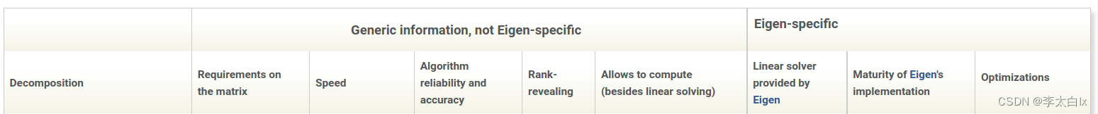
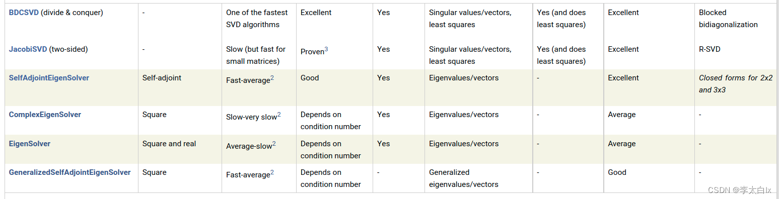
第二列是这些方法对矩阵的要求,第三列是计算的速度,第四列是算法的可靠性与准确性。
3.1 个人总结
BDCSVD和JacobiSVD是计算奇异值的,如果维度小于16, 可以直接用JacobiSVD。
SelfAdjointEigenSolver是计算实对称矩阵或者复数下的自伴矩阵的特征值与特征向量的。
ComplexEigenSolver是计算复数矩阵的特征值与特征向量的。
EigenSolver是一般矩阵(非对称矩阵,复数矩阵)的特征值与特征向量。
GeneralizedSelfAdjointEigenSolver 是计算 Av = λBv用的,需要输入2个矩阵,A是自伴矩阵,B是正定矩阵,然后计算出特征值λ和特征向量v。