目录
- 一、问题描述
- 二、图像预处理
- 2.1 中值滤波去噪
- 2.2 白平衡处理
- 三、焊缝边缘检测
- 3.1 Sobel算子边缘检测
- 3.2 Prewitt算子边缘检测
- 3.3 Canny算子边缘检测
- 3.4 形态学处理边缘检测
- 四、结果分析
一、问题描述
目前很多机械关键部件均为钢焊接结构,钢焊接结构易出现裂纹、漏焊、焊缝外观不规则等缺陷,因此对焊缝质量检测尤为重要。焊缝边缘是焊缝图像最重要的特征,经典的边缘提取算法通过考虑相连像素间的灰度变化,利用边缘邻接第一或第二阶导数的变化规律来实现边缘提取。在常用的一些边缘检测算子中,Sobel常常形成不封闭的区域,其他算子例如Laplace算子通常产生重响应。**本文采用T型焊接焊缝图像进行分析,讨论了基于形态学处理的焊缝边缘检测方法,该算法信噪比大且精度高。**该算法首先采用中值滤波、白平衡处理、图像归一化处理等图像预处理技术纠正采集图像,然后采用形态学处理算法提取焊缝的二值化图,该算法不仅有效的降噪,而且保证图像有用信息不丢失。焊缝图像如下:
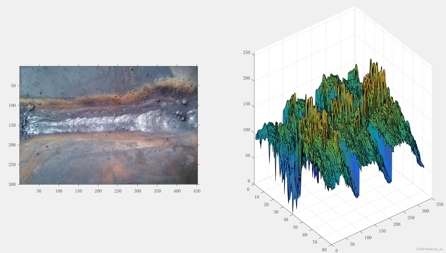
代码如下:
clear
close all;
ps=imread('1.jpg');
subplot(121),imshow(ps)
background=imopen(ps,strel('disk',4));
% imshow(background);
subplot(122),surf(double(background(1:4:end,1:4:end))),zlim([0 256]);
set(gca,'Ydir','reverse');
二、图像预处理
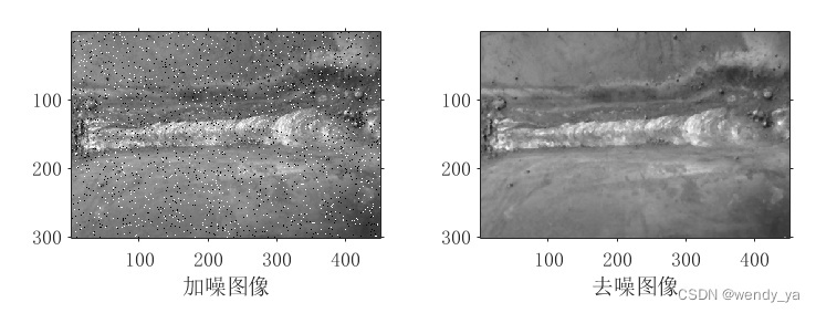
2.1 中值滤波去噪
中值滤波是一种邻域运算,类似于卷积,信号中值是按信号值大小顺序排列后的中间值,采用中值滤波可以较好地消除脉冲干扰和保持信号边缘。代码如下:
%% 读取焊缝图像
clc,clear,close all
obj=imread('1.jpg');
r=obj(:,:,1);g=obj(:,:,2);b=obj(:,:,3);
%% 去噪中值滤波
objn=imnoise(g,'salt & pepper',0.04);%加入少许椒盐噪声
K1=medfilt2(objn,[3,3]);%3x3模板中值滤波
K2=medfilt2(objn,[5,5]);%5x5模板中值滤波
figure('color',[1,1,1])
subplot(121),imshow(objn);xlabel('加噪图像')
subplot(122),imshow(K1);xlabel('去噪图像')
运行结果:
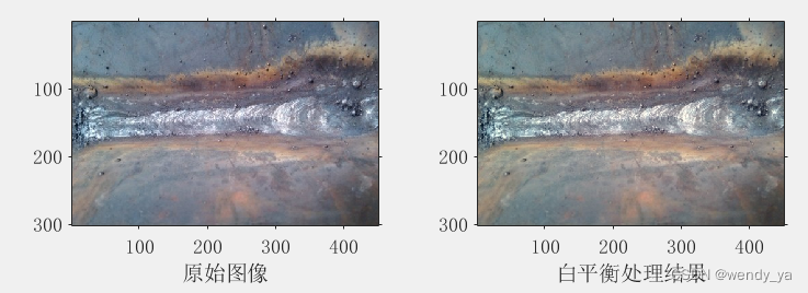
2.2 白平衡处理
由于拍摄图像存在大量噪声,往往使图像中所有物体的颜色都偏离了它们原有的真实色彩,采用白平衡方法处理图像失真,从而校正有色片的图像颜色,以获得正常颜色的图像。代码如下:
clc,clear,close all
img=imread('1.jpg');
subplot(121),imshow(img),xlabel('原始图像')
img_1=img(:,:,1);
img_2=img(:,:,2);
img_3=img(:,:,3);
Y=0.299*img_1+0.587*img_2+0.114*img_3;  % 白平衡系数
[m,n]=size(Y);
k=Y(1,1);
for i=1:m
    for j=1:n
        if Y(i,j)>=k
            k=Y(i,j);
            k1=i;
            k2=j;
        end
    end
end
[m1,n1]=find(Y==k);
Rave=sum(sum(img_1));
Rave=Rave/(m*n);
Gave=sum(sum(img_2));
Gave=Gave/(m*n);
Bave=sum(sum(img_3));
Bave=Bave/(m*n);
Kave=(Rave+Gave+Bave)/3;
img__1=(Kave/Rave)*img_1;
img__2=(Kave/Gave)*img_2;
img__3=(Kave/Bave)*img_3;
imgysw=cat(3,img__1,img__2,img__3);
subplot(122),imshow(imgysw),xlabel('白平衡处理结果')
运行结果:
三、焊缝边缘检测
图像边缘是图像中灰度不连续或急剧变化的所有像素的集合,集中了图像的大部分信息,是图像最基本的特征之一。边缘检测是后续的图像分割、特征提取和识别等图像分析领域关键性的一步,在工程应用中有着十分重要的地位。传统检测法通过计算图像各个像素点的一阶或二阶微分来确定边缘,图像一阶微分的峰值点或二阶微分的过零点对应图像的边缘像素点,较常见的检测算子有:Sobel、Prewitt和Canny等算子。
3.1 Sobel算子边缘检测
Sobel算子是把图像中的每个像素的上下左右四邻域的灰度值加权差,在边缘处达到机制从而检测边缘。其定义为:
S
x
=
[
f
(
x
+
1
,
y
−
1
)
+
2
f
(
x
+
1
,
y
)
+
f
(
x
+
1
,
y
+
1
)
]
−
[
f
(
x
−
1
,
y
−
1
)
+
2
f
(
x
−
1
,
y
)
+
f
(
x
−
1
,
y
+
1
)
]
{S_x} = \left[ {f\left( {x + 1{\rm{,}}y{\rm{ - }}1} \right) + 2f\left( {x + 1{\rm{,}}y} \right) + f\left( {x + 1{\rm{,}}y + 1} \right)} \right]{\rm{ - }}\left[ {f\left( {x{\rm{ - }}1{\rm{,}}y{\rm{ - }}1} \right) + 2f\left( {x{\rm{ - }}1{\rm{,}}y} \right) + f\left( {x{\rm{ - }}1{\rm{,}}y + 1} \right)} \right]
Sx=[f(x+1,y−1)+2f(x+1,y)+f(x+1,y+1)]−[f(x−1,y−1)+2f(x−1,y)+f(x−1,y+1)]
S
y
=
[
f
(
x
−
1
,
y
+
1
)
+
2
f
(
x
,
y
+
1
)
+
f
(
x
+
1
,
y
+
1
)
]
−
[
f
(
x
−
1
,
y
−
1
)
+
2
f
(
x
,
y
−
1
)
+
f
(
x
+
1
,
y
−
1
)
]
{S_y} = \left[ {f\left( {x{\rm{ - }}1{\rm{,}}y + 1} \right) + 2f\left( {x{\rm{,}}y + 1} \right) + f\left( {x + 1{\rm{,}}y + 1} \right)} \right]{\rm{ - }}\left[ {f\left( {x{\rm{ - }}1{\rm{,}}y{\rm{ - }}1} \right) + 2f\left( {x{\rm{,}}y{\rm{ - }}1} \right) + f\left( {x + 1{\rm{,}}y{\rm{ - }}1} \right)} \right]
Sy=[f(x−1,y+1)+2f(x,y+1)+f(x+1,y+1)]−[f(x−1,y−1)+2f(x,y−1)+f(x+1,y−1)]
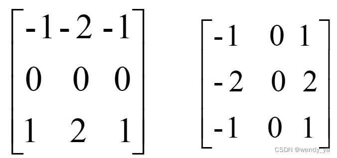
图像中每个像素点都与下面两个核做卷积,一个核对垂直边缘影响最大,而另一个核对水平边缘影响最大,两个卷积的最大值作为这个像素点的输出值。Sobel算子卷积模板为:
Sobel算子代码如下:
%% Sobel
clc,clear,close all
I=imread('1.jpg'); % 读入图像
r=I(:,:,1);g=I(:,:,2);b=I(:,:,3);
nI=size(r);
im = single(I) / 255;
yfilter = fspecial('sobel'); % sobel
xfilter = yfilter';
rx = imfilter(im(:,:,1), xfilter);
gx = imfilter(im(:,:,2), xfilter);
bx = imfilter(im(:,:,3), xfilter);
ry = imfilter(im(:,:,1), yfilter);
gy = imfilter(im(:,:,2), yfilter);
by = imfilter(im(:,:,3), yfilter);
Jx = rx.^2 + gx.^2 + bx.^2;
Jy = ry.^2 + gy.^2 + by.^2;
Jxy = rx.*ry + gx.*gy + bx.*by;
D = sqrt(abs(Jx.^2 - 2*Jx.*Jy + Jy.^2 + 4*Jxy.^2)); % 2x2 matrix J'*J的第一个特征值
e1 = (Jx + Jy + D) / 2;
% e2 = (Jx + Jy - D) / 2; %第二个特征值
edge_magnitude = sqrt(e1);
edge_orientation = atan2(-Jxy, e1 - Jy);
% figure,
% subplot(121),imshow(edge_magnitude)
% subplot(122),imshow(edge_orientation)
sob=edge(edge_magnitude,'sobel',0.29);
% sob=bwareaopen(sob,100);
% figure,imshow(y),title('Sobel Edge Detection')
% 3*3 sobel
f=edge_magnitude;
sx=[-1 0 1;-2 0 2;-1 0 1]; % 卷积模板convolution mask
sy=[-1 -2 -1;0 0 0;1 2 1]; % 卷积模板convolution mask
for x=2:1:nI(1,1)-1
for y=2:1:nI(1,2)-1
mod=[f(x-1,y-1),2*f(x-1,y),f(x-1,y+1);
f(x,y-1),2*f(x,y),f(x,y+1);
f(x+1,y-1),2*f(x+1,y),f(x+1,y+1)];
mod=double(mod);
fsx=sx.*mod;
fsy=sy.*mod;
ftemp(x,y)=sqrt((sum(fsx(:)))^2+(sum(fsy(:)))^2);
end
end
fs=im2bw(ftemp); % fs=im2uint8(ftemp);
fs=bwareaopen(fs,500);
% figure,imshow(fs);title('Sobel Edge Detection')
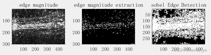
subplot(131),imshow(edge_magnitude),title('edge magnitude')
subplot(132),imshow(sob),title('edge magnitude extraction')
subplot(133),imshow(fs);title('sobel Edge Detection')
运行结果:
3.2 Prewitt算子边缘检测
Prewitt算子将边缘检测算子模板的大小从2x2扩大到3x3,进行差分算子的计算,将方向差分算子与局部平均相结合,从而减小噪声对图像边缘检测的影响。其定义为:
S
x
=
[
f
(
x
−
1
,
y
+
1
)
+
f
(
x
,
y
+
1
)
+
f
(
x
+
1
,
y
+
1
)
]
−
[
f
(
x
−
1
,
y
−
1
)
−
f
(
x
,
y
−
1
)
−
f
(
x
+
1
,
y
−
1
)
]
{S_x} = \left[ {f\left( {x{\rm{ - }}1{\rm{,}}y + 1} \right) + f\left( {x{\rm{,}}y + 1} \right) + f\left( {x + 1{\rm{,}}y + 1} \right)} \right]{\rm{ - }}\left[ {f\left( {x{\rm{ - }}1{\rm{,}}y{\rm{ - }}1} \right){\rm{ - }}f\left( {x{\rm{,}}y{\rm{ - }}1} \right){\rm{ - }}f\left( {x + 1{\rm{,}}y{\rm{ - }}1} \right)} \right]
Sx=[f(x−1,y+1)+f(x,y+1)+f(x+1,y+1)]−[f(x−1,y−1)−f(x,y−1)−f(x+1,y−1)]
S
y
=
[
f
(
x
+
1
,
y
−
1
)
+
f
(
x
+
1
,
y
)
+
f
(
x
+
1
,
y
+
1
)
]
−
[
f
(
x
−
1
,
y
−
1
)
−
f
(
x
−
1
,
y
)
−
f
(
x
−
1
,
y
+
1
)
]
{S_y} = \left[ {f\left( {x + 1{\rm{,}}y{\rm{ - }}1} \right) + f\left( {x + 1{\rm{,}}y} \right) + f\left( {x + 1{\rm{,}}y + 1} \right)} \right]{\rm{ - }}\left[ {f\left( {x{\rm{ - }}1{\rm{,}}y{\rm{ - }}1} \right){\rm{ - }}f\left( {x{\rm{ - }}1{\rm{,}}y} \right){\rm{ - }}f\left( {x{\rm{ - }}1{\rm{,}}y + 1} \right)} \right]
Sy=[f(x+1,y−1)+f(x+1,y)+f(x+1,y+1)]−[f(x−1,y−1)−f(x−1,y)−f(x−1,y+1)]
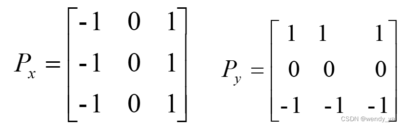
Prewitt算子的卷积模板为:
G
(
i
,
j
)
=
∣
P
x
∣
+
∣
P
y
∣
G(i,j)=|P_x|+|P_y|
G(i,j)=∣Px∣+∣Py∣,式中:
Prewitt算子代码如下:
%% Prewitt
clc,clear,close all
I=imread('1.jpg'); % 读入图像
r=I(:,:,1);g=I(:,:,2);b=I(:,:,3);
nI=size(r);
im = single(I) / 255;
yfilter = fspecial('prewitt'); % prewitt
xfilter = yfilter';
rx = imfilter(im(:,:,1), xfilter);
gx = imfilter(im(:,:,2), xfilter);
bx = imfilter(im(:,:,3), xfilter);
ry = imfilter(im(:,:,1), yfilter);
gy = imfilter(im(:,:,2), yfilter);
by = imfilter(im(:,:,3), yfilter);
Jx = rx.^2 + gx.^2 + bx.^2;
Jy = ry.^2 + gy.^2 + by.^2;
Jxy = rx.*ry + gx.*gy + bx.*by;
D = sqrt(abs(Jx.^2 - 2*Jx.*Jy + Jy.^2 + 4*Jxy.^2)); % 2x2 matrix J'*J的第一个特征值
e1 = (Jx + Jy + D) / 2;
% e2 = (Jx + Jy - D) / 2; %第二个特征值
edge_magnitude = sqrt(e1);
edge_orientation = atan2(-Jxy, e1 - Jy);
% figure,
% subplot(121),imshow(edge_magnitude)
% subplot(122),imshow(edge_orientation)
pre=edge(edge_magnitude,'prewitt',0.19);
% figure,imshow(y),title('Prewitt Edge Detection')
% 3*3 prewitt
f=edge_magnitude;
sx=[-1 0 1;-1 0 1;-1 0 1]; % convolution mask
sy=[1 1 1;0 0 0;-1 -1 -1]; % convolution mask
for x=2:1:nI(1,1)-1
for y=2:1:nI(1,2)-1
mod=[f(x-1,y-1),f(x-1,y),f(x-1,y+1);
f(x,y-1),f(x,y),f(x,y+1);
f(x+1,y-1),f(x+1,y),f(x+1,y+1)];
mod=double(mod);
fsx=sx.*mod;
fsy=sy.*mod;
ftemp(x,y)=sqrt((sum(fsx(:)))^2+(sum(fsy(:)))^2);
end
end
fs=im2bw(ftemp); % fs=im2uint8(ftemp);
fs=bwareaopen(fs,1000);
% figure,imshow(fs);title('Prewitt Edge Detection');
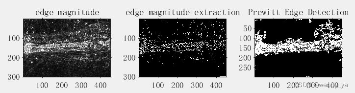
subplot(131),imshow(edge_magnitude),title('edge magnitude')
subplot(132),imshow(pre),title('edge magnitude extraction')
subplot(133),imshow(fs);title('Prewitt Edge Detection');
运行结果:
3.3 Canny算子边缘检测
传统的Canny算法采用2x2邻域一阶偏导的有限差分来计算平滑后的数据阵列I(x,y)的梯度幅值和梯度方向。定义为:
P
x
(
i
,
j
)
=
(
I
(
i
,
j
+
1
)
−
I
(
i
,
j
)
+
I
(
i
+
1
,
j
+
1
)
−
I
(
i
+
1
,
j
)
)
/
2
{P_x}\left( {i,j} \right) = \left( {I\left( {i,j + 1} \right) - I\left( {i,j} \right) + I\left( {i + 1,j + 1} \right) - I\left( {i + 1,j} \right)} \right)/2
Px(i,j)=(I(i,j+1)−I(i,j)+I(i+1,j+1)−I(i+1,j))/2
P
y
(
i
,
j
)
=
(
I
(
i
,
j
)
−
I
(
i
+
1
,
j
)
+
I
(
i
,
j
+
1
)
−
I
(
i
+
1
,
j
+
1
)
)
/
2
{P_y}\left( {i,j} \right) = \left( {I\left( {i,j} \right) - I\left( {i + 1,j} \right) + I\left( {i,j + 1} \right) - I\left( {i + 1,j + 1} \right)} \right)/2
Py(i,j)=(I(i,j)−I(i+1,j)+I(i,j+1)−I(i+1,j+1))/2
像素的梯度幅值和梯度方向用直角坐标到极坐标的坐标转化公式来计算,用二阶范数来计算梯度幅值为:
M
(
i
,
j
)
=
P
x
(
i
,
j
)
2
+
P
y
(
i
,
j
)
2
M\left( {i,j} \right) = \sqrt {{P_x}{{\left( {i,j} \right)}^2} + {P_y}{{\left( {i,j} \right)}^2}}
M(i,j)=Px(i,j)2+Py(i,j)2
梯度方向为:
θ
[
i
,
j
]
=
arctan
(
P
y
(
i
,
j
)
/
P
x
j
(
i
,
j
)
)
\theta \left[ {i,j} \right] = \arctan \left( {{P_y}\left( {i,j} \right)/{P_{xj}}\left( {i,j} \right)} \right)
θ[i,j]=arctan(Py(i,j)/Pxj(i,j))
Canny算子进行图像边缘检测是较为有效的,检测样本边缘的噪声和焊接位置是精确的,但是焊缝表面质量纹理较为规则,Canny检测纹理较细,增加了计算工作量,对噪声影响较大。代码如下:
%% Canny
clc,clear,close all
im=imread('1.jpg');  % 载入图像
im=im2double(im);
r=im(:,:,1);g=im(:,:,2);b=im(:,:,3);
% 滤波器平滑系数
filter= [2 4 5 4 2;
         4 9 12 9 4;
         5 12 15 12 5;
         4 9 12 9 4;
         2 4 5 4 2];
filter=filter/115;
% N-dimensional convolution
smim= convn(im,filter);
% imshow(smim);title('Smoothened image');

% 计算梯度
gradXfilt=[-1 0 1; % 卷积模板convolution mask
           -2 0 2;
           -1 0 1];
gradYfilt=[1  2   1; % 卷积模板 convolution mask
           0  0   0;
          -1  -2  -1];
GradX= convn(smim,gradXfilt);
GradY= convn(smim,gradYfilt);
absgrad=abs(GradX)+abs(GradY);
% computing angle of gradients
[a,b]=size(GradX);
theta=zeros([a b]);
for i=1:a
      for j=1:b
            if(GradX(i,j)==0)
               theta(i,j)=atan(GradY(i,j)/0.000000000001);
            else
                theta(i,j)=atan(GradY(i,j)/GradX(i,j));
            end
      end
 end
  theta=theta*(180/3.14);
  for i=1:a
      for j=1:b
            if(theta(i,j)<0)
                theta(i,j)= theta(i,j)-90;
                theta(i,j)=abs(theta(i,j));
            end
      end
 end
  for i=1:a
      for j=1:b
          if ((0<theta(i,j))&&(theta(i,j)<22.5))||((157.5<theta(i,j))&&(theta(i,j)<181))
                theta(i,j)=0;
          elseif (22.5<theta(i,j))&&(theta(i,j)<67.5)
                 theta(i,j)=45;
          elseif (67.5<theta(i,j))&&(theta(i,j)<112.5)
                  theta(i,j)=90;
          elseif (112.5<theta(i,j))&&(theta(i,j)<157.5)
                  theta(i,j)=135;
          end
      end
  end

%non-maximum suppression
nmx = padarray(absgrad, [1 1]);
[a,b]=size(theta);
for i=2:a-2
    for j=2:b-2
           if (theta(i,j)==135)
                 if ((nmx(i-1,j+1)>nmx(i,j))||(nmx(i+1,j-1)>nmx(i,j)))
                      nmx(i,j)=0;
                  end
           elseif (theta(i,j)==45)
                  if ((nmx(i+1,j+1)>nmx(i,j))||(nmx(i-1,j-1)>nmx(i,j)))
                       nmx(i,j)=0;
                  end
           elseif (theta(i,j)==90)
                  if ((nmx(i,j+1)>nmx(i,j))||(nmx(i,j-1)>nmx(i,j)))
                      nmx(i,j)=0;
                  end
           elseif (theta(i,j)==0)
                  if ((nmx(i+1,j)>nmx(i,j))||(nmx(i-1,j)>nmx(i,j)))
                      nmx(i,j)=0;
                  end
           end
    end
end

nmx1=im2uint8(nmx); % 图像数据类型转换
tl=85;  % 阈值下限lower threshold
th=100; % 阈值上限upper threshold

% grouping edges based on threshold
[a,b]=size(nmx1);
gedge=zeros([a,b]);
for i=1:a
    for j=1:b
        if(nmx1(i,j)>th)
             gedge(i,j)=nmx1(i,j);
        elseif (tl<nmx1(i,j))&&(nmx1(i,j)<th)
             gedge(i,j)=nmx1(i,j);
        end
    end
end

[a,b]= size(gedge);
finaledge=zeros([a b]);
for i=1:a
    for j=1:b
        if (gedge(i,j)>th)
            finaledge(i,j)=gedge(i,j);
             for i2=(i-1):(i+1)
                 for j2= (j-1):(j+1)
                     if (gedge(i2,j2)>tl)&&(gedge(i2,j2)<th)
                         finaledge(i2,j2)=gedge(i,j);
                     end
                 end
              end
        end
   end
end

%clearing the border
finaledge= im2uint8(finaledge(10:end-10,10:end-10));

subplot(131);imshow(absgrad);title('image gradients');
subplot(132);imshow(nmx);title('NonMaximum Suppression');
subplot(133);imshow(finaledge(:,1:452-10));title('canny edge detection');
运行结果:

3.4 形态学处理边缘检测
形态学处理边缘检测的流程如下:
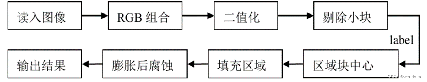
运行结果如下:
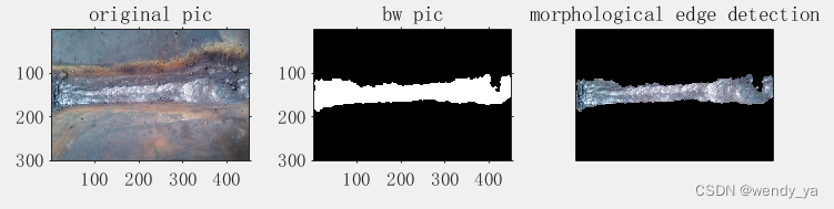
四、结果分析
由上图可知,Sobel 算子对图像边缘进行检测,其检测结果较细致,背景轮廓干扰太大,以至于不能对目标焊缝进行单一提取。;Prewitt 算子对图像边缘具有较好的提取作用,但是焊缝受背景影响较大,提取的效果较差,提取边缘没有闭合的区域;Canny 算子基于双阈值的非极大值抑制,得到边缘图像,较之于Sobel 和Prewit算子,检测纹理较细,但由于没有形成闭合的区域,对于剔除背景边缘,单独提取焊缝轮廓,仍较难操作;采用形态学边缘检测,对图像噪声过滤较好,得到的二值化图像接近于实际目标,保证了焊缝特征信息的不丢失,从而能很好地提取焊缝特征, 信噪比大且精度高。
ok,以上便是本文的全部内容了,完整代码可以参考:https://download.csdn.net/download/didi_ya/87743384;如果对你有所帮助,记得点个赞哟~