一、简介和环境准备
knn一般指邻近算法。 邻近算法,或者说K最邻近(KNN,K-NearestNeighbor)分类算法是数据挖掘分类技术中最简单的方法之一。而lmknn是局部均值k最近邻分类算法。
本次实验环境需要用的是Google Colab和Google Drive(云盘),文件后缀是.ipynb可以直接用。首先登录谷歌云盘(网页),再打卡ipynb文件就可以跳转到谷歌colab了。再按以下点击顺序将colab和云盘链接。
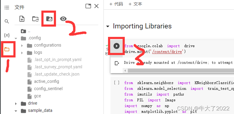
from google.colab import drive
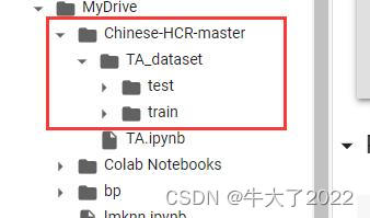
drive.mount('/content/drive')准备的数据是一些分类好的手写汉字图(实验来源在结尾)
引入库
from sklearn.neighbors import KNeighborsClassifier
from sklearn.model_selection import train_test_split
from imutils import paths
from PIL import Image
import numpy as np
import matplotlib.pyplot as plt
import glob
import argparse
import imutils
import cv2
import os
# import sys
# np.set_printoptions(threshold=sys.maxsize)
二、数据预处理和算法简介
2.1预处理
注意路径的修改。这一步处理所有图片数据,存到xy的train和test。
x_train = []
y_train = []
x_test = []
y_test = []

for i in os.listdir('./drive/MyDrive/Chinese-HCR-master/TA_dataset/train'):
    for filename in glob.glob('drive/MyDrive/Chinese-HCR-master/TA_dataset/train/'+str(i)+'/*.png'):
        im = cv2.imread(filename, 0)
        im = cv2.resize(im, (128, 128)) # resize to 128 * 128 pixel size
        blur = cv2.GaussianBlur(im, (5,5), 0) # using Gaussian blur
        ret, th = cv2.threshold(blur, 0, 255, cv2.THRESH_BINARY + cv2.THRESH_OTSU)
        x_train.append(th)
        y_train.append(i) # append class

for i in os.listdir('./drive/MyDrive/Chinese-HCR-master/TA_dataset/test'):
    for filename in glob.glob('drive/MyDrive/Chinese-HCR-master/TA_dataset/test/'+str(i)+'/*.png'):
        im = cv2.imread(filename, 0)
        im = cv2.resize(im, (128, 128)) # resize to 128 * 128 pixel size
        blur = cv2.GaussianBlur(im, (5,5), 0) # using Gaussian blur
        ret, th = cv2.threshold(blur, 0, 255, cv2.THRESH_BINARY + cv2.THRESH_OTSU)
        x_test.append(th)
        y_test.append(i) # append class
x_train = np.array(x_train) / 255
x_test = np.array(x_test) / 255
y_train = np.array(y_train)
# x_train = np.array(x_train)
# x_test = np.array(x_test)可以打印看一下
plt.imshow(x_train[0])
plt.show()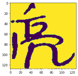
plt.imshow(x_test[0], 'gray')
plt.show()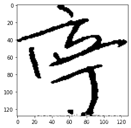
2.2算法代码
1.KNN
这里不像上一章分析源码,只调用
from sklearn.neighbors import KNeighborsClassifier
from sklearn.metrics import accuracy_score
neigh = KNeighborsClassifier(n_neighbors=3)
xtrain = np.reshape(x_train, (x_train.shape[0], x_train.shape[1] * x_train.shape[1]))
xtest = np.reshape(x_test, (x_test.shape[0], x_test.shape[1] * x_test.shape[1]))prediction = neigh.fit(xtrain, y_train).predict(xtrain)
prediction
print(accuracy_score(y_train,prediction))0.7969348659003831
2.基于HOG特征提取的KNN
from skimage.feature import hogfeatures = np.array(xtrain, 'int64')
labels = y_trainlist_hog_fd = []
for feature in features:
fd = hog(
feature.reshape((128, 128)),
orientations=8,
pixels_per_cell=(64, 64),
cells_per_block=(1, 1), )
list_hog_fd.append(fd)hog_features = np.array(list_hog_fd)
hog_featuresarray([[0.52801754, 0. , 0.52801754, ..., 0. , 0.5 , 0. ], [0.35309579, 0. , 0.54016151, ..., 0. , 0.5 , 0. ], [0.5 , 0. , 0.5 , ..., 0. , 0.5 , 0. ], ..., [0.5035908 , 0. , 0.59211517, ..., 0. , 0.5 , 0. ], [0.51920317, 0. , 0.51920317, ..., 0. , 0.5 , 0. ], [0.55221191, 0. , 0.55221191, ..., 0. , 0.5 , 0. ]])
(注:如果没运行1的knn 要先跑下面的)
neigh = KNeighborsClassifier(n_neighbors=3)
xtrain = np.reshape(x_train, (x_train.shape[0], x_train.shape[1] * x_train.shape[1]))
xtest = np.reshape(x_test, (x_test.shape[0], x_test.shape[1] * x_test.shape[1]))
prediction = neigh.fit(hog_features, labels).predict(hog_features)
prediction
print(accuracy_score(labels,prediction))0.6360153256704981
3.带骨架的KNN
from skimage.morphology import skeletonize
from skimage import data
import matplotlib.pyplot as plt
from skimage.util import invert
# Invert the horse image
image = invert(x_train[0])
# perform skeletonization
skeleton = skeletonize(image)
# display results
fig, axes = plt.subplots(nrows=1, ncols=2, figsize=(8, 4),
sharex=True, sharey=True)
ax = axes.ravel()
ax[0].imshow(image, cmap=plt.cm.gray)
ax[0].axis('off')
ax[0].set_title('original', fontsize=20)
ax[1].imshow(skeleton, cmap=plt.cm.gray)
ax[1].axis('off')
ax[1].set_title('skeleton', fontsize=20)
fig.tight_layout()
plt.show()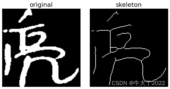
from sklearn.neighbors import KNeighborsClassifier
neigh = KNeighborsClassifier(n_neighbors=3)
xtrain = np.reshape(x_train, (x_train.shape[0], x_train.shape[1] * x_train.shape[1]))
xtest = np.reshape(x_test, (x_test.shape[0], x_test.shape[1] * x_test.shape[1]))from sklearn.metrics import accuracy_score
prediction = neigh.fit(xtrain, y_train).predict(xtrain)
prediction
print(accuracy_score(y_train,prediction))
0.7969348659003831
4.拓展--Otsu方法概述
import cv2 as cv
import numpy as np
from matplotlib import pyplot as plt
img = cv.imread('drive/MyDrive/Chinese-HCR-master/TA_dataset/train/亮/37162.png',0)
img = cv.medianBlur(img,5)
ret,th1 = cv.threshold(img,127,255,cv.THRESH_BINARY)
th2 = cv.adaptiveThreshold(img,255,cv.ADAPTIVE_THRESH_MEAN_C,\
            cv.THRESH_BINARY,11,2)
th3 = cv.adaptiveThreshold(img,255,cv.ADAPTIVE_THRESH_GAUSSIAN_C,\
            cv.THRESH_BINARY,11,2)
titles = ['Original Image', 'Global Thresholding (v = 127)',
            'Adaptive Mean Thresholding', 'Adaptive Gaussian Thresholding']
images = [img, th1, th2, th3]
for i in range(4):
    plt.subplot(2,2,i+1),plt.imshow(images[i],'gray')
    plt.title(titles[i])
    plt.xticks([]),plt.yticks([])
plt.show()
import cv2 as cv
import numpy as np
from matplotlib import pyplot as plt
img = cv.imread('drive/MyDrive/Chinese-HCR-master/TA_dataset/train/亮/37162.png',0)
# global thresholding
ret1,th1 = cv.threshold(img,127,255,cv.THRESH_BINARY)
# Otsu's thresholding
ret2,th2 = cv.threshold(img,0,255,cv.THRESH_BINARY+cv.THRESH_OTSU)
# Otsu's thresholding after Gaussian filtering
blur = cv.GaussianBlur(img,(5,5),0)
ret3,th3 = cv.threshold(blur,0,255,cv.THRESH_BINARY+cv.THRESH_OTSU)
# plot all the images and their histograms
images = [img, 0, th1,
          img, 0, th2,
          blur, 0, th3]
titles = ['Original Noisy Image','Histogram','Global Thresholding (v=127)',
          'Original Noisy Image','Histogram',"Otsu's Thresholding",
          'Gaussian filtered Image','Histogram',"Otsu's Thresholding"]
for i in range(3):
    plt.subplot(3,3,i*3+1),plt.imshow(images[i*3],'gray')
    plt.title(titles[i*3]), plt.xticks([]), plt.yticks([])
    plt.subplot(3,3,i*3+2),plt.hist(images[i*3].ravel(),256)
    plt.title(titles[i*3+1]), plt.xticks([]), plt.yticks([])
    plt.subplot(3,3,i*3+3),plt.imshow(images[i*3+2],'gray')
    plt.title(titles[i*3+2]), plt.xticks([]), plt.yticks([])
plt.show()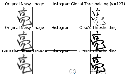
来源:GitHub - NovitaGuok/Chinese-HCR: A Chinese Character Recognition system using KNN, LMPNN, and MVMCNN


![3.知识图谱概念和相关技术简介[知识抽取、知识融合、知识推理方法简述],典型应用案例介绍国内落地产品介绍。一份完整的入门指南,带你快速掌握KG知识,芜湖起飞!](https://img-blog.csdnimg.cn/190ddc3c7454438ea0ffd435c81f9423.png)