0. 简介

作为SLAM中常用的方法，其原因是因为SLAM观测不只考虑到当前帧的情况，而需要加入之前状态量的观测。就比如一个在二维平面上移动的机器人，机器人可以使用一组传感器，例如车轮里程计或激光测距仪。从这些原始测量值中，我们想要估计机器人的轨迹并构建环境地图。为了降低问题的计算复杂度，位姿图方法将原始测量值抽象出来。具体来说，它创建了一个表示机器人姿态的节点图，以及表示两个节点之间的相对变换（增量位置和方向）的边。边缘是源自原始传感器测量值的虚拟测量值，例如通过集成原始车轮里程计或对齐从机器人获取的激光范围扫描。
在这里插入图片描述
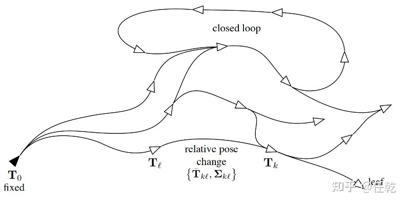
对上图的具体描述如下

1. Ceres-Solver的位姿图优化

1.1 Ceres-Solver的用法

之前作者已经已经在《SLAM本质剖析-Ceres》中详细的介绍了SLAM中对Ceres的使用。使用 Ceres Solver求解非线性优化问题，主要包括以下几部分：

构建代价函数(cost function)或残差(residual)
构建优化问题(ceres::Problem)：通过 AddResidualBlock 添加代价函数(cost function)、损失函数(loss function核函数) 和待优化状态量
配置求解器(ceres::Solver::Options)
运行求解器(ceres::Solve(options, &problem, &summary))

与g2o优化中直接在边上添加information（信息矩阵）不同，Ceres无法直接实现此功能。 由于Ceres只接受最小二乘优化就，即 $min(r^{^{T}}r)$ ;若要对残差加权，使用马氏距离即 $(r^{^{T}}\Sigma r)$ ,则要对信息矩阵（协方差矩阵） $\Sigma$ 做Cholesky分解： $LL^{^{T}}=\Sigma$ ，则 $r^{^{T}}\Sigma r=r^{^{T}}(LL^{^{T}})r=(L^{^{T}}r)^{T}(L^{T}r)$ ，令 $r'=L^{T}r$ ,最终得到纯种的最小二乘优化： $min(r'^{^{T}}r')$ 。

1.2 Ceres优化步骤

这一块的内容在前文中已经详细阐述了，这里就不详细分析了，下面直接贴一下每个部分的代码以及结构的组成。

Step1：构建Cost Function

（1）AutoDiffCostFunction（自动求导）

构造 代价函数结构体或代价函数类（例如：struct CostFunctor），在其结构体内对模板括号() 重载用来定义残差；
在重载的 () 函数形参中，**最后一个为残差，前面几个为待优化状态量，注意：**形参类型必须是模板类型。

struct CostFunctor {
    template<typename T>
    bool operator()(const T *const x, T *residual) const {
        residual[0] = 10.0 - x[0]; // r(x) = 10 - x
        return true;
    }
};

利用ceres::CostFunction *cost_function=new ceres::AutoDiffCostFunction<functype,dimension1,dimension2>(new costFunc)，获得Cost Function

模板参数分别是：代价结构体仿函数类型名，残差维度，第一个优化变量维度，第二个…；函数参数（new costFunc）是代价结构体（或类）对象，即此对象重载的 () 函数的函数指针

（2）NumericDiffCostFunction（数值求导）

数值求导法 也是构造 代价函数结构体，也需要重载括号()来定义残差，但在重载括号() 时没有用模板；

struct CostFunctorNum {
    bool operator()(const double *const x, double *residual) const {
        residual[0] = 10.0 - x[0]; // r(x) = 10 - x
        return true;
    }
};

并且在实例化代价函数时也稍微有点区别，多了一个模板参数 ceres::CENTRAL

ceres::CostFunction *cost_function;
cost_function =new ceres::NumericDiffCostFunction<CostFunctorNum, ceres::CENTRAL, 1, 1>(new CostFunctorNum);

（3）自定义CostFunction

构建一个继承自 ceres::SizedCostFunction<1,1> 的类，同样，对于模板参数的数字，第一个为残差的维度，后面几个为待优化状态量的维度 ；
重载虚函数virtual bool Evaluate(double const* const* parameters, double *residuals, double **jacobians) const，根据待优化变量，实现 残差和雅克比矩阵的计算（雅克比矩阵计算需要提供公式）；

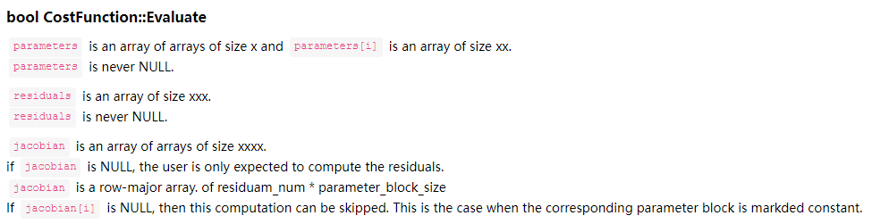
virtual bool Evaluate(double const* const* parameters, double* residuals, double** jacobians) const；：核心函数，跟自动求导中用仿函数中 operator() 类似，这里重写了基类中的 evaluate 函数，并且需要在其中定义误差和雅克比矩阵的计算方式：
double const* const* parameters：参数块，主要是传入的各个节点，第一维度为节点的个数（这里是 6），第二维度则是对应节点的维度（这里两个节点的维度都是 6）
double* residuals：残差，维度取决于误差的维度，这里是 6
double** jacobians：雅克比矩阵，第一个维度为节点的个数（也就是要求解的雅克比矩阵的数量），第二个维度为对应雅克比矩阵的元素个数（这里两个雅克比矩阵的维度都是 6x6，因此维度是 36）
详细的解析可以看一下这篇博客Ceres 学习记录（一）：2D 位姿图优化


class PoseGraphCFunc : public ceres::SizedCostFunction<6,6,6>
{
public:
    EIGEN_MAKE_ALIGNED_OPERATOR_NEW;
    PoseGraphCFunc(const Sophus::SE3 measure,const Matrix6d covariance):_measure(measure),_covariance(covariance){}
    ~PoseGraphCFunc(){}
    virtual bool Evaluate(double const* const* parameters,
                          double *residuals,
                          double **jacobians)const
    {
    	//创建带有参数的SE3
        Sophus::SE3 pose_i=Sophus::SE3::exp(Vector6d(parameters[0]));//Eigen::MtatrixXd可以通过double指针来构造
        Sophus::SE3 pose_j=Sophus::SE3::exp(Vector6d(parameters[1]));
        Eigen::Map<Vector6d> residual(residuals);//Eigen::Map<typename MatrixX>(ptr)函数的作用是通过传入指针将c++数据映射为Eigen上的Matrix数据，有点与&相似
        //通过LLT分解得到信息矩阵
        residual=(_measure.inverse()*pose_i.inverse()*pose_j).log();
        Matrix6d sqrt_info=Eigen::LLT<Matrix6d>(_covariance).matrixLLT().transpose();
        //计算雅克比矩阵
        if(jacobians)
        {
            if(jacobians[0])
            {
                Eigen::Map<Eigen::Matrix<double,6,6,Eigen::RowMajor>> jacobian_i(jacobians[0]);
                Matrix6d Jr=JRInv(Sophus::SE3::exp(residual));
                jacobian_i=(sqrt_info)*(-Jr)*pose_j.inverse().Adj();
            }
            if(jacobians[1])
            {
                Eigen::Map<Eigen::Matrix<double,6,6, Eigen::RowMajor>> jacobian_j(jacobians[1]);
                Matrix6d J = JRInv(Sophus::SE3::exp(residual));
                jacobian_j = sqrt_info * J * pose_j.inverse().Adj();
            }
        }
        residual=sqrt_info*residual;
        return true;

    }
private:
    const Sophus::SE3 _measure;
    const Matrix6d _covariance;

};

如果待优化变量处于流形上则需自定义一个继承于LocalParameterization的类，重载其中的Plus()函数实现迭代递增，重载computeJacobian()定义流形到切平面的雅克比矩阵


class Parameterization:public ceres::LocalParameterization
{
public:
    Parameterization(){}
    virtual ~Parameterization(){}
    virtual bool Plus(const double* x,
                      const double * delta,
                      double *x_plus_delta)const
    {
        Vector6d lie(x);
        Vector6d lie_delta(delta);
        Sophus::SE3 T=Sophus::SE3::exp(lie);
        Sophus::SE3 T_delta=Sophus::SE3::exp(lie_delta);

        Eigen::Map<Vector6d> x_plus(x_plus_delta);
        x_plus=(T_delta*T).log();
        return true;

    }
    //流形到其切平面的雅克比矩阵
    virtual bool ComputeJacobian(const double *x,
                                 double * jacobian) const
    {
        ceres::MatrixRef(jacobian,6,6)=ceres::Matrix::Identity(6,6);//ceres::MatrixRef()函数也类似于Eigen::Map,通过模板参数传入C++指针将c++数据映射为Ceres::Matrix
        return true;
    }
    //定义流形和切平面维度：在本问题中是李代数到李代数故都为6
    virtual int GlobalSize()const{return 6;}
    virtual int LocalSize()const {return 6;}
};

Step2:AddResidualBlock

声明 ceres::Problem problem;
通过 AddResidualBlock 将 代价函数(cost function)、损失函数(loss function) 和待优化状态量 添加到 problem

ceres::LossFunction *loss = new ceres::HuberLoss(1.0);
ceres::CostFunction *costfunc = new PoseGraphCFunc(measurement, covariance);//定义costfunction
problem.AddResidualBlock(costfunc, loss, param[vertex_i].se3, param[vertex_j].se3);//为整体代价函数加入快，ceres的优点就是直接在param[vertex_i].se3上优化
problem.SetParameterization(param[vertex_i].se3, local_param);//为待优化的两个位姿变量定义迭代递增方式
problem.SetParameterization(param[vertex_j].se3, local_param);

Step3:配置优化参数并优化Config&solve

定义ceres::Solver::Options options;对options成员进行赋值以配置优化参数；
定义ceres::Solver::Summary summary;用来存储优化输出；
求解：ceres::Solve(options, &problem, &summary);

ceres::Solver::Options options;//配置优化设置
options.linear_solver_type = ceres::SPARSE_NORMAL_CHOLESKY;
options.trust_region_strategy_type=ceres::LEVENBERG_MARQUARDT;
options.max_linear_solver_iterations = 50;
options.minimizer_progress_to_stdout = true;
ceres::Solver::Summary summary;//summary用来存储优化过程
ceres::Solve(options, &problem, &summary);//开始优化

1.3 Ceres代码详解

这里借鉴了这篇文章的信息。并结合自己的理解去进行分析，解决了作者未能解决的问题。

1.3.1.pose_graph_2d_error_term.h

这个文件中主要是实现了ceres计算残差需要的类，也就是之前自己定义的包含模板()运算符的结构体或类。并且在这个类的定义中，官方注释非常详细的解释了残差的计算公式，结合官网的教程很容易明白。

// Computes the error term for two poses that have a relative pose measurement
// between them. Let the hat variables be the measurement.
//
// residual =  information^{1/2} * [  r_a^T * (p_b - p_a) - \hat{p_ab}   ]
//                                 [ Normalize(yaw_b - yaw_a - \hat{yaw_ab}) ]
//
// where r_a is the rotation matrix that rotates a vector represented in frame A
// into the global frame, and Normalize(*) ensures the angles are in the range
// [-pi, pi).
class PoseGraph2dErrorTerm {
 public:
  PoseGraph2dErrorTerm(double x_ab,   // 这些都是实际观测值，也就是位姿图中的边
                       double y_ab,
                       double yaw_ab_radians,
                       const Eigen::Matrix3d& sqrt_information)
      : p_ab_(x_ab, y_ab),
        yaw_ab_radians_(yaw_ab_radians),
        sqrt_information_(sqrt_information) {}

  template <typename T>
   // 括号运算符中传入的是节点的值，然后利用这些值计算估计的观测值，
   // 和实际传入的观测值做差，得到残差
  bool operator()(const T* const x_a,  
                  const T* const y_a,
                  const T* const yaw_a,
                  const T* const x_b,
                  const T* const y_b,
                  const T* const yaw_b,
                  T* residuals_ptr) const {
    const Eigen::Matrix<T, 2, 1> p_a(*x_a, *y_a);
    const Eigen::Matrix<T, 2, 1> p_b(*x_b, *y_b);

    // 为什么要声明为Map呢？经常操作，并且给它赋值的数据是Eigen的数据类型？
    // map就像相当于C++中的数组，主要是为了和原生的C++数组交互
    Eigen::Map<Eigen::Matrix<T, 3, 1>> residuals_map(residuals_ptr);  

    residuals_map.template head<2>() =
        RotationMatrix2D(*yaw_a).transpose() * (p_b - p_a) - p_ab_.cast<T>();
    residuals_map(2) = ceres::examples::NormalizeAngle(
        (*yaw_b - *yaw_a) - static_cast<T>(yaw_ab_radians_));

    // Scale the residuals by the square root information matrix to account for
    // the measurement uncertainty.
    residuals_map = sqrt_information_.template cast<T>() * residuals_map;

    return true;
  }

  // 再次看到static，只是为了提高程序紧凑型，因为下面这个函数只给当前这个类用，类似一种全局函数
  static ceres::CostFunction* Create(double x_ab,
                                     double y_ab,
                                     double yaw_ab_radians,
                                     const Eigen::Matrix3d& sqrt_information) {
    return (new ceres::
                AutoDiffCostFunction<PoseGraph2dErrorTerm, 3, 1, 1, 1, 1, 1, 1>(
                    new PoseGraph2dErrorTerm(
                        x_ab, y_ab, yaw_ab_radians, sqrt_information)));
  }

  EIGEN_MAKE_ALIGNED_OPERATOR_NEW

 private:
  // The position of B relative to A in the A frame.
  const Eigen::Vector2d p_ab_;
  // The orientation of frame B relative to frame A.
  const double yaw_ab_radians_;
  // The inverse square root of the measurement covariance matrix.
  const Eigen::Matrix3d sqrt_information_;
};

注意上面程序中的几个细节：

还是原来的套路，类的形参传入的是实际观测的数据点，也就是g2o中的边，传入的这些数据值会赋值给类的成员变量，在()运算中计算残差的时候会用到这些成员变量，也就是观测的数据值。而对于()运算符，传入的是顶点的值，就是g2o中的顶点，或者说是要被优化的值。然后在()运算中，先利用这些顶点值得到计算的观测值，然后和实际的观测值相减，就得到了残差。
这个类中再次出现了static函数，这个函数就是返回new出来的一个自动求导对象指针。这样写在类里的好处是让程序更加紧凑，因为自动求导对象里的构造参数是和我们定义的这个类数据紧密相关的。
在()运算中定义残差的时候，使用到了eigen中的map类。实际上map类是为了兼容eigen的矩阵操作与C++的数组操作。
（1）看程序中有一句EIGEN_MAKE_ALIGNED_OPERATOR_NEW声明内存对齐，这在自定义的类中使用Eigen的数据类型时是必要的，还有的时候能看到在std::vector中插入Eigen的变量后面要加一个Eigen::Aligend...，也是为了声明Eigen的内存对齐，这样才能使用STL容器。所以这里要清楚，Eigen为了实现矩阵运算，其内存和原生的C++内存分配出现了差别，很多时候都需要声明一下。
（2）再回到map类，这个类就是为了实现和C++中数组一样的内存分配方式，比如使用指针可以快速访问；但是同时他又可以支持Eigen的矩阵运算，所以在需要对矩阵元素频繁操作或者访问的时候，声明为map类是一个很好的选择。再来看这里为什么要声明为map类？首先频繁操作，要把算出来的残差存到这个矩阵中；其次计算的结果（=右边）都是eigen的数据类型，所以也要和Eigen的数据类型兼容。所以满足使用map的两个情况，因此使用map类很合适。
（3）详细资料参见：Eigen库中的Map类到底是做什么的
(4) map.template中template是由于block是模板化成员，如果矩阵类型也是模板参数，则必须使用关键字模板

residuals_map.template head<2>() =
        RotationMatrix2D(*yaw_a).transpose() * (p_b - p_a) - p_ab_.cast<T>();
    residuals_map(2) = ceres::examples::NormalizeAngle(
        (*yaw_b - *yaw_a) - static_cast<T>(yaw_ab_radians_));

1.3.2.pose_graph_2d.h

这个文件就是主文件，主要就是实现添加残差块。对于每一个观测数据，都需要添加残差块。然后其中还有官网说的那个Normalize限制旋转角度的范围的问题。

其次还有一个比较重要的问题，就是程序中最后把最开始的那个位姿设置成了常量，不优化它，也就是那段长注释解释的，具体我没有看的很懂。

// The pose graph optimization problem has three DOFs that are not fully  
// constrained. This is typically referred to as gauge freedom. You can apply  
// a rigid body transformation to all the nodes and the optimization problem  
// will still have the exact same cost. The Levenberg-Marquardt algorithm has  
// internal damping which mitigate this issue, but it is better to properly  
// constrain the gauge freedom. This can be done by setting one of the poses  
// as constant so the optimizer cannot change it.

位姿图优化问题具有三个未完全约束的自由度。这通常称为规范自由度。您可以对所有节点应用刚体变换，优化问题仍然具有完全相同的成本。 Levenberg-Marquardt 算法具有内部阻尼来缓解这个问题，但最好适当地约束规范自由度。这可以通过将其中一个姿势设置为常量来完成，这样优化器就无法更改它。

// Constructs the nonlinear least squares optimization problem from the pose
// graph constraints.
// Constraint2d 2D的约束，是一个自定义的结构体类，描述了顶点之间的位姿约束，也就是g2o中的边
void BuildOptimizationProblem(const std::vector<Constraint2d>& constraints,
                              std::map<int, Pose2d>* poses,
                              ceres::Problem* problem) {
  CHECK(poses != NULL);
  CHECK(problem != NULL);
  if (constraints.empty()) {
    LOG(INFO) << "No constraints, no problem to optimize.";
    return;
  }
  // LossFunction就是和函数，这里不使用核函数
  ceres::LossFunction* loss_function = NULL;
  // 局部参数化：
  // Lastly, we use a local parameterization to normalize the orientation in the range which is normalized between【-pi,pi)
  ceres::LocalParameterization* angle_local_parameterization =
      AngleLocalParameterization::Create();

  // 使用常量迭代器访问容器，得到容器中的所有元素
  for (std::vector<Constraint2d>::const_iterator constraints_iter =
           constraints.begin();
       constraints_iter != constraints.end();
       ++constraints_iter) {
    const Constraint2d& constraint = *constraints_iter;  // 得到当前访问的约束元素

    std::map<int, Pose2d>::iterator pose_begin_iter =
        poses->find(constraint.id_begin);  // 根据约束的顶点Id号得到指向顶点1的迭代器
    CHECK(pose_begin_iter != poses->end())  // 找到了
        << "Pose with ID: " << constraint.id_begin << " not found.";
    std::map<int, Pose2d>::iterator pose_end_iter = // 根据约束的顶点Id号得到指向顶点2的迭代器
        poses->find(constraint.id_end);
    CHECK(pose_end_iter != poses->end())
        << "Pose with ID: " << constraint.id_end << " not found.";

    const Eigen::Matrix3d sqrt_information =
            // llt = LL^T，cholesky分解，然后matrixL是cholesky因子组成的矩阵
        constraint.information.llt().matrixL();  // 信息矩阵，即协方差矩阵的逆
    // Ceres will take ownership of the pointer.
    // PoseGraph2dErrorTerm是专门定义的一个用于2D位姿图优化的类，相当于这个类中已经定义好了残差块的()运算符
    // 和之前自己写计算残差的结构体或者类是一样的。costfunction是添加参数块的时候必须使用的
    ceres::CostFunction* cost_function = PoseGraph2dErrorTerm::Create(
        constraint.x, constraint.y, constraint.yaw_radians, sqrt_information);
    // 对每一个观测值，都添加残差块
    problem->AddResidualBlock(cost_function,
                              loss_function,
                              &pose_begin_iter->second.x,  // 因为这是一个map的迭代器，map中first就是key值，second就是value值
                              &pose_begin_iter->second.y,  // 因为key存的是pose的id号，这里用的是顶点的pose，所以是value的值
                              &pose_begin_iter->second.yaw_radians,
                              &pose_end_iter->second.x,
                              &pose_end_iter->second.y,
                              &pose_end_iter->second.yaw_radians);

    // 设置参数化，这里设置边的两个顶点的pose的旋转角度为 local_parameterization
    problem->SetParameterization(&pose_begin_iter->second.yaw_radians,
                                 angle_local_parameterization);
    problem->SetParameterization(&pose_end_iter->second.yaw_radians,
                                 angle_local_parameterization);
  }

  // The pose graph optimization problem has three DOFs that are not fully
  // constrained. This is typically referred to as gauge freedom. You can apply
  // a rigid body transformation to all the nodes and the optimization problem
  // will still have the exact same cost. The Levenberg-Marquardt algorithm has
  // internal damping which mitigate this issue, but it is better to properly
  // constrain the gauge freedom. This can be done by setting one of the poses
  // as constant so the optimizer cannot change it.
  std::map<int, Pose2d>::iterator pose_start_iter = poses->begin();
  CHECK(pose_start_iter != poses->end()) << "There are no poses.";
  problem->SetParameterBlockConstant(&pose_start_iter->second.x);
  problem->SetParameterBlockConstant(&pose_start_iter->second.y);
  problem->SetParameterBlockConstant(&pose_start_iter->second.yaw_radians);
}

2. G2O的位姿图优化

G2O这部分也在我们的系列文章《SLAM本质剖析-G2O》中详细的阐述了。这里不详细的去写了。G2O本身就是经常被用于位姿图优化的，所以这里我们直接给出例子。算法的整个流程：1、构造g2o优化问题并执行优化；2、每次优化完成后，对地图点是否为外点进行卡方检验，检验到为内点的加入下次优化，否则下次不优化；3、得到优化后的当前帧的位姿（此函数只优化当前帧位姿）