PyTorch学习笔记（一）：PyTorch环境安装

往期学习资料推荐：

1.Pytorch实战笔记_GoAI的博客-CSDN博客

2.Pytorch入门教程_GoAI的博客-CSDN博客

安装参考：

1.视频教程：3分钟深度学习【环境搭建】CUDA +Anaconda 简单粗暴_哔哩哔哩】

2.windows10下CUDA11.1、cuDNN8.0、tensorflow-gpu2.4.1安装教程以及问题解决方法_3.Win10中CUDA、cuDNN的安装与卸载

4.Pytorch详细安装-强推！

1.安装CUDA

安装包下载地址（主博客在介绍版本选择的时候也有提到）
官网各种version的CUDA下载地址
官网各种cuDNN下载地址
打开“cuda_8.0.44_win10.exe”，此过程会很慢，耐心等待（这也提示我该换电脑了）

选择解压地址（反正是临时的，就C盘吧，问题不大）

开始解压（此过程依然很慢，特别是我的电脑那段时间不知道出了什么问题CPU和内存占用异常高，这个过程也是费了我很多时间）
解压完毕，加在安装程序
开始安装
4. 敲黑板了！这里千万不要选默认的精简，这里的精简应该改成全部才对（看下面的小字说明，这就是全家桶），倒不是说安装全家桶不可以，主要是有一个东西的安装会一直导致安装失败
特别是这个visual studio integration千万不能选！

选择以下的安装就够了

就装在C盘吧，之后别的地方路径啥的会方便一点
安装成功
验证安装成功
（1）环境变量应该已经自动加好

（2）cmd里查看版本信息nvcc -V
（3）进入到路径下后查看GPU运行时的监测界面
（4）运行bandwidthTest.exe（需要先进入到所在目录）

（5）运行deviceQuery.exe（需要先进入到所在目录）

2.安装cuDNN

官网各种cuDNN下载地址
cuDNN称不上安装，只需要将下载下来的压缩包解压后，将对应文件夹的文件放到CUDA安装路径下的对应文件夹里即可
在这里插入图片描述

3.卸载

cuDNN本来就只是将文件拷贝进CUDA的安装目录，故删除即可（卸载CUDA后直接删除整个文件夹也可以）
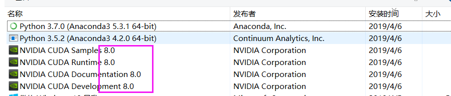
CUDA的卸载：控制面板-卸载程序（不要用360等杀毒软件，找不到对应程序的），按照安装时间排序，最上面这几个带版本号的，就是刚才安装的CUDA了，挨个卸载即可
在这里插入图片描述

PyTorch学习笔记（二）：PyTorch简介与基础知识

1. PyTorch简介

概念：由Facebook人工智能研究小组开发的一种基于Lua编写的Torch库的Python实现的深度学习库
优势：简洁、上手快、具有良好的文档和社区支持、项目开源、支持代码调试、丰富的扩展库

2 PyTorch基础知识

2.1张量

分类：0维张量（标量）、1维张量（向量）、2维张量（矩阵）、3维张量（时间序列）、4维张量（图像）、5维张量（视频）
概念：一个数据容器，可以包含数据、字符串等

import torch
# 创建tensor
x = torch.rand(4, 3)
print(x)
# 构造数据类型为long，数据是0的矩阵
x = torch.zeros(4, 3, dtype=torch.long)
print(x)

tensor([[0.9515, 0.6332, 0.8228],
        [0.3508, 0.0493, 0.7606],
        [0.7326, 0.7003, 0.1925],
        [0.1172, 0.8946, 0.9501]])
tensor([[0, 0, 0],
        [0, 0, 0],
        [0, 0, 0],
        [0, 0, 0]])

常见的构造Tensor的函数：

函数	功能
Tensor(*sizes)	基础构造函数
tensor(data)	类似于np.array
ones(*sizes)	全1
zeros(*sizes)	全0
eye(*sizes)	对角为1，其余为0
arange(s,e,step)	从s到e，步长为step
linspace(s,e,steps)	从s到e，均匀分成step份
rand/randn(*sizes)	rand是[0,1)均匀分布；randn是服从N（0，1）的正态分布
normal(mean,std)	正态分布（均值为mean，标准差是std）
randperm(m)	随机排列

操作：
1. 使用索引表示的变量与原数据共享内存，即修改其中一个，另一个也会被修改
2. 使用torch.view改变tensor的大小
3. 广播机制：当对两个形状不同的Tensor按元素运算时，可能会触发广播(broadcasting)机制

# 使用view改变张量的大小
x = torch.randn(5, 4)
y = x.view(20)
z = x.view(-1, 5) # -1是指这一维的维数由其他维度决定
print(x.size(), y.size(), z.size())

torch.Size([5, 4]) torch.Size([20]) torch.Size([4, 5])

x = tensor([[1, 2]])
y = tensor([[1],
        [2],
        [3]])
x + y = tensor([[2, 3],
        [3, 4],
        [4, 5]])

2.2 自动求导

autograd包：提供张量上的自动求导机制
原理：如果设置.requires_grad为True，那么将会追踪张量的所有操作。当完成计算后，可以通过调用.backward()自动计算所有的梯度。张量的所有梯度将会自动累加到.grad属性
Function：Tensor和Function互相连接生成了一个无环图 (acyclic graph)，它编码了完整的计算历史。每个张量都有一个.grad_fn属性，该属性引用了创建Tensor自身的Function

x = torch.ones(2, 2, requires_grad=True)
print(x)
tensor([[1., 1.],
        [1., 1.]], requires_grad=True)
y = x ** 2
print(y)
tensor([[1., 1.],
        [1., 1.]], grad_fn=<PowBackward0>)
z = y * y * 3
out = z.mean()
print("z = ", z)
print("z mean = ", out)
z =  tensor([[3., 3.],
        [3., 3.]], grad_fn=<MulBackward0>)
z mean =  tensor(3., grad_fn=<MeanBackward0>)

grad的反向传播：运行反向传播，梯度都会累加之前的梯度，所以一般在反向传播之前需把梯度清零

out.backward()
print(x.grad)
tensor([[3., 3.],
        [3., 3.]])
# 反向传播累加
out2 = x.sum()
out2.backward()
print(x.grad)
tensor([[4., 4.],
        [4., 4.]])

2.3并行计算

目的：通过使用多个GPU参与训练，加快训练速度，提高模型学习的效果
CUDA：通过使用NVIDIA提供的GPU并行计算框架，采用cuda()方法，让模型或者数据迁移到GPU中进行计算
并行计算方法：
1. Network partitioning：将一个模型网络的各部分拆分，分配到不同的GPU中,执行不同的计算任务
2. Layer-wise partitioning：将同一层模型拆分，分配到不同的GPU中，训练同一层模型的部分任务
3. Data parallelism（主流）：将不同的数据分配到不同的GPU中，执行相同的任务

PyTorch学习笔记（三）：PyTorch主要组成模块

往期学习资料推荐：

1.Pytorch实战笔记_GoAI的博客-CSDN博客

2.Pytorch入门教程_GoAI的博客-CSDN博客

1 深度学习步骤

（1）数据预处理：通过专门的数据加载，通过批训练提高模型表现，每次训练读取固定数量的样本输入到模型中进行训练
（2）深度神经网络搭建：逐层搭建，实现特定功能的层（如积层、池化层、批正则化层、LSTM层等）
（3）损失函数和优化器的设定：保证反向传播能够在用户定义的模型结构上实现
（4）模型训练：使用并行计算加速训练，将数据按批加载，放入GPU中训练，对损失函数反向传播回网络最前面的层，同时使用优化器调整网络参数

2 基本配置

导入相关的包

import os
import numpy as py
import torch
import torch.nn as nn
from torch.utils.data 
import Dataset, DataLoader
import torch.optim as optimizer

统一设置超参数：batch size、初始学习率、训练次数、GPU配置

# set batch size
batch_size = 16
 
# 初始学习率
lr = 1e-4
 
# 训练次数
max_epochs = 100
 
# 配置GPU
device = torch.device("cuda:1" if torch.cuda.is_available() else "cpu")
device
 
device(type='cuda', index=1)

3 数据读入

读取方式：通过Dataset+DataLoader的方式加载数据，Dataset定义好数据的格式和数据变换形式，DataLoader用iterative的方式不断读入批次数据。
自定义Dataset类：实现__init___、__getitem__、__len__函数
torch.utils.data.DataLoader参数：
1. batch_size：样本是按“批”读入的，表示每次读入的样本数
2. num_workers：表示用于读取数据的进程数
3. shuffle：是否将读入的数据打乱
4. drop_last：对于样本最后一部分没有达到批次数的样本，使其不再参与训练

4 模型构建

4.1 神经网络的构造

通过Module类构造模型，实例化模型之后，可完成模型构造

# 构造多层感知机
class MLP(nn.Module):
    def __init__(self, **kwargs):
        super(MLP, self).__init__(**kwargs)
        self.hidden = nn.Linear(784, 256)
        self.act = nn.ReLU()
        self.output = nn.Linear(256, 10)
        
    def forward(self, X):
        o = self.act(self.hidden(x))
        return self.output(o)
 
x = torch.rand(2, 784)
net = MLP()
print(x)
net(x)

tensor([[0.8924, 0.9624, 0.3262,  ..., 0.8376, 0.1889, 0.9060],
        [0.3609, 0.8005, 0.5175,  ..., 0.6255, 0.1462, 0.9846]])
 
 
 
 
 
tensor([[-0.0902,  0.0199,  0.0677, -0.0679,  0.0799,  0.0826,  0.0628,  0.1809,
         -0.2387,  0.0366],
        [-0.2271,  0.0056, -0.0984, -0.0432, -0.0160, -0.0038,  0.0953,  0.0545,
         -0.1530, -0.0214]], grad_fn=<AddmmBackward>)

4.2 神经网络常见的层

不含模型参数的层

# 构造一个输入减去均值后输出的层
class MyLayer(nn.Module):
    def __init__(self, **kwargs):
        super(MyLayer, self).__init__(**kwargs)
    
    def forward(self, x):
        return x - x.mean()
x = torch.tensor([0, 5, 10, 15, 20], dtype=torch.float)
layer = MyLayer()
layer(x)

tensor([-10.,  -5.,   0.,   5.,  10.])

含模型参数的层：如果一个Tensor是Parameter，那么它会⾃动被添加到模型的参数列表里

# 使用ParameterList定义参数的列表
class MyListDense(nn.Module):
    def __init__(self):
        super(MyListDense, self).__init__()
        self.params = nn.ParameterList(
            [nn.Parameter(torch.randn(4, 4)) for i in range(3)])
        self.params.append(nn.Parameter(torch.randn(4, 1)))
 
    def forward(self, x):
        for i in range(len(self.params)):
            x = torch.mm(x, self.params[i])
        return x
net = MyListDense()
print(net)

MyListDense(
  (params): ParameterList(
      (0): Parameter containing: [torch.FloatTensor of size 4x4]
      (1): Parameter containing: [torch.FloatTensor of size 4x4]
      (2): Parameter containing: [torch.FloatTensor of size 4x4]
      (3): Parameter containing: [torch.FloatTensor of size 4x1]
  )
)

# 使用ParameterDict定义参数的字典
class MyDictDense(nn.Module):
    def __init__(self):
        super(MyDictDense, self).__init__()
        self.params = nn.ParameterDict({
                'linear1': nn.Parameter(torch.randn(4, 4)),
                'linear2': nn.Parameter(torch.randn(4, 1))
        })
        # 新增参数linear3
        self.params.update({'linear3': nn.Parameter(torch.randn(4, 2))}) 
 
    def forward(self, x, choice='linear1'):
        return torch.mm(x, self.params[choice])
 
net = MyDictDense()
print(net)

MyDictDense(
  (params): ParameterDict(
      (linear1): Parameter containing: [torch.FloatTensor of size 4x4]
      (linear2): Parameter containing: [torch.FloatTensor of size 4x1]
      (linear3): Parameter containing: [torch.FloatTensor of size 4x2]
  )
)

二维卷积层：使用nn.Conv2d类构造，模型参数包括卷积核和标量偏差，在训练模式时，通常先对卷积核随机初始化，再不断迭代卷积核和偏差

# 计算卷积层，对输入和输出做相应的升维和降维
def comp_conv2d(conv2d, X):
    # (1, 1)代表批量大小和通道数
    X = X.view((1, 1) + X.shape)
    Y = conv2d(X)
    # 排除不关心的前两维：批量和通道
    return Y.view(Y.shape[2:]) 
# 注意这里是两侧分别填充1⾏或列，所以在两侧一共填充2⾏或列
conv2d = nn.Conv2d(in_channels=1, out_channels=1, kernel_size=3,padding=1)
 
X = torch.rand(8, 8)
comp_conv2d(conv2d, X).shape

torch.Size([8, 8])

池化层：直接计算池化窗口内元素的最大值或者平均值，分别叫做最大池化或平均池化

# 二维池化层
def pool2d(X, pool_size, mode='max'):
    p_h, p_w = pool_size
    Y = torch.zeros((X.shape[0] - p_h + 1, X.shape[1] - p_w + 1))
    for i in range(Y.shape[0]):
        for j in range(Y.shape[1]):
            if mode == 'max':
                Y[i, j] = X[i: i + p_h, j: j + p_w].max()
            elif mode == 'avg':
                Y[i, j] = X[i: i + p_h, j: j + p_w].mean()
    return Y
X = torch.tensor([[0, 1, 2], [3, 4, 5], [6, 7, 8]], dtype=torch.float)
pool2d(X, (2, 2), 'max')

tensor([[4., 5.],
        [7., 8.]])

pool2d(X, (2, 2), 'avg')

tensor([[2., 3.],
        [5., 6.]])

4.3 模型示例

神经网络训练过程：
1. 定义可学习参数的神经网络
2. 在输入数据集上进行迭代训练
3. 通过神经网络处理输入数据
4. 计算loss（损失值）
5. 将梯度反向传播给神经网络参数
6. 更新网络参数，使用梯度下降
LeNet(前馈神经网络)

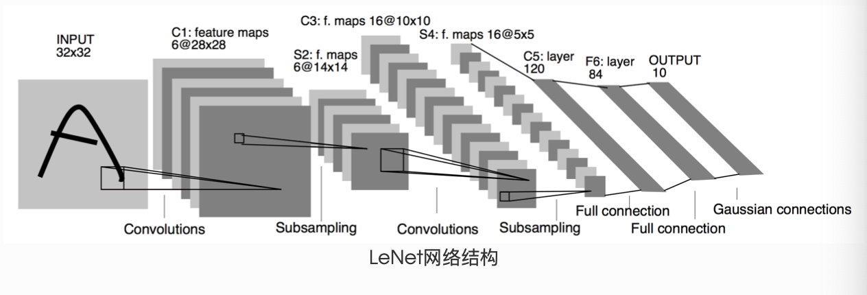
import torch.nn.functional as F
 
class Net(nn.Module):
    def __init__(self):
        super(Net, self).__init__()
        # 输入图像channel是1；输出channel是6；5x5卷积核
        self.conv1 = nn.Conv2d(1, 6, 5)
        self.conv2 = nn.Conv2d(6, 16, 5)
        # an affine operation: y = Wx + b
        self.fc1 = nn.Linear(16 * 5 * 5, 120)
        self.fc2 = nn.Linear(120, 84)
        self.fc3 = nn.Linear(84, 10)
 
    def forward(self, x):
        # 2x2 Max pooling
        x = F.max_pool2d(F.relu(self.conv1(x)), (2, 2))
        # 如果是方阵,则可以只使用一个数字进行定义
        x = F.max_pool2d(F.relu(self.conv2(x)), 2)
        x = x.view(-1, self.num_flat_features(x))
        x = F.relu(self.fc1(x))
        x = F.relu(self.fc2(x))
        x = self.fc3(x)
        return x
 
    def num_flat_features(self, x):
        # 除去批处理维度的其他所有维度
        size = x.size()[1:]  
        num_features = 1
        for s in size:
            num_features *= s
        return num_features
 
net = Net()
net

Net(
  (conv1): Conv2d(1, 6, kernel_size=(5, 5), stride=(1, 1))
  (conv2): Conv2d(6, 16, kernel_size=(5, 5), stride=(1, 1))
  (fc1): Linear(in_features=400, out_features=120, bias=True)
  (fc2): Linear(in_features=120, out_features=84, bias=True)
  (fc3): Linear(in_features=84, out_features=10, bias=True)
)

# 假设输入的数据为随机的32x32
input = torch.randn(1, 1, 32, 32)
out = net(input)
print(out)

tensor([[-0.0921, -0.0605, -0.0726, -0.0451,  0.1399, -0.0087,  0.1075,  0.0799,
         -0.1472,  0.0288]], grad_fn=<AddmmBackward>)

# 清零所有参数的梯度缓存，然后进行随机梯度的反向传播
net.zero_grad()
out.backward(torch.randn(1, 10))

AlexNet

class AlexNet(nn.Module):
    def __init__(self):
        super(AlexNet, self).__init__()
        self.conv = nn.Sequential(
            # in_channels, out_channels, kernel_size, stride, padding
            nn.Conv2d(1, 96, 11, 4), 
            nn.ReLU(),
            # kernel_size, stride
            nn.MaxPool2d(3, 2), 
            # 减小卷积窗口，使用填充为2来使得输入与输出的高和宽一致，且增大输出通道数
            nn.Conv2d(96, 256, 5, 1, 2),
            nn.ReLU(),
            nn.MaxPool2d(3, 2),
            # 连续3个卷积层，且使用更小的卷积窗口。
            # 除了最后的卷积层外，进一步增大了输出通道数。
            # 前两个卷积层后不使用池化层来减小输入的高和宽
            nn.Conv2d(256, 384, 3, 1, 1),
            nn.ReLU(),
            nn.Conv2d(384, 384, 3, 1, 1),
            nn.ReLU(),
            nn.Conv2d(384, 256, 3, 1, 1),
            nn.ReLU(),
            nn.MaxPool2d(3, 2)
        )
         # 这里全连接层的输出个数比LeNet中的大数倍。使用丢弃层来缓解过拟合
        self.fc = nn.Sequential(
            nn.Linear(256*5*5, 4096),
            nn.ReLU(),
            nn.Dropout(0.5),
            nn.Linear(4096, 4096),
            nn.ReLU(),
            nn.Dropout(0.5),
            # 输出层。由于这里使用Fashion-MNIST，所以用类别数为10，而非论文中的1000
            nn.Linear(4096, 10),
        )
 
    def forward(self, img):
        feature = self.conv(img)
        output = self.fc(feature.view(img.shape[0], -1))
        return output
net = AlexNet()
print(net)

AlexNet(
  (conv): Sequential(
    (0): Conv2d(1, 96, kernel_size=(11, 11), stride=(4, 4))
    (1): ReLU()
    (2): MaxPool2d(kernel_size=3, stride=2, padding=0, dilation=1, ceil_mode=False)
    (3): Conv2d(96, 256, kernel_size=(5, 5), stride=(1, 1), padding=(2, 2))
    (4): ReLU()
    (5): MaxPool2d(kernel_size=3, stride=2, padding=0, dilation=1, ceil_mode=False)
    (6): Conv2d(256, 384, kernel_size=(3, 3), stride=(1, 1), padding=(1, 1))
    (7): ReLU()
    (8): Conv2d(384, 384, kernel_size=(3, 3), stride=(1, 1), padding=(1, 1))
    (9): ReLU()
    (10): Conv2d(384, 256, kernel_size=(3, 3), stride=(1, 1), padding=(1, 1))
    (11): ReLU()
    (12): MaxPool2d(kernel_size=3, stride=2, padding=0, dilation=1, ceil_mode=False)
  )
  (fc): Sequential(
    (0): Linear(in_features=6400, out_features=4096, bias=True)
    (1): ReLU()
    (2): Dropout(p=0.5, inplace=False)
    (3): Linear(in_features=4096, out_features=4096, bias=True)
    (4): ReLU()
    (5): Dropout(p=0.5, inplace=False)
    (6): Linear(in_features=4096, out_features=10, bias=True)
  )
)

5 损失函数

二分类交叉熵损失函数：torch.nn.BCELoss，用于计算二分类任务时的交叉熵

m = nn.Sigmoid()
loss = nn.BCELoss()
input = torch.randn(3, requires_grad=True)
target = torch.empty(3).random_(2)
 
output = loss(m(input), target)
output.backward()
print('BCE损失函数的计算结果:',output)

BCE损失函数的计算结果: tensor(0.9389, grad_fn=<BinaryCrossEntropyBackward>)

交叉熵损失函数：torch.nn.CrossEntropyLoss，用于计算交叉熵

loss = nn.CrossEntropyLoss()
input = torch.randn(3, 5, requires_grad=True)
target = torch.empty(3, dtype=torch.long).random_(5)
 
output = loss(input, target)
output.backward()
print('CrossEntropy损失函数的计算结果:',output)

CrossEntropy损失函数的计算结果: tensor(2.7367, grad_fn=<NllLossBackward>)

L1损失函数：torch.nn.L1Loss，用于计算输出y和真实值target之差的绝对值

loss = nn.L1Loss()
input = torch.randn(3, 5, requires_grad=True)
target = torch.randn(3, 5)
 
output = loss(input, target)
output.backward()
print('L1损失函数的计算结果:',output)

L1损失函数的计算结果: tensor(1.0351, grad_fn=<L1LossBackward>)

MSE损失函数：torch.nn.MSELoss，用于计算输出y和真实值target之差的平方

loss = nn.MSELoss()
input = torch.randn(3, 5, requires_grad=True)
target = torch.randn(3, 5)
 
output = loss(input, target)
output.backward()
print('MSE损失函数的计算结果:',output)

MSE损失函数的计算结果: tensor(1.7612, grad_fn=<MseLossBackward>)

平滑L1（Smooth L1）损失函数：torch.nn.SmoothL1Loss，用于计算L1的平滑输出，减轻离群点带来的影响，通过与L1损失的比较，在0点的尖端处，过渡更为平滑

loss = nn.SmoothL1Loss()
input = torch.randn(3, 5, requires_grad=True)
target = torch.randn(3, 5)
 
output = loss(input, target)
output.backward()
print('Smooth L1损失函数的计算结果:',output)

Smooth L1损失函数的计算结果: tensor(0.7252, grad_fn=<SmoothL1LossBackward>)

目标泊松分布的负对数似然损失：torch.nn.PoissonNLLLoss

loss = nn.PoissonNLLLoss()
log_input = torch.randn(5, 2, requires_grad=True)
target = torch.randn(5, 2)
 
output = loss(log_input, target)
output.backward()
print('PoissonNL损失函数的计算结果:',output)

PoissonNL损失函数的计算结果: tensor(1.7593, grad_fn=<MeanBackward0>)

KL散度：torch.nn.KLDivLoss，用于连续分布的距离度量，可用在对离散采用的连续输出空间分布的回归场景

inputs = torch.tensor([[0.5, 0.3, 0.2], [0.2, 0.3, 0.5]])
target = torch.tensor([[0.9, 0.05, 0.05], [0.1, 0.7, 0.2]], dtype=torch.float)
loss = nn.KLDivLoss(reduction='batchmean')
 
output = loss(inputs,target)
print('KLDiv损失函数的计算结果:',output)

KLDiv损失函数的计算结果: tensor(-1.0006)

MarginRankingLoss：torch.nn.MarginRankingLoss，用于计算两组数据之间的差异（相似度），可使用在排序任务的场景

= nn.MarginRankingLoss() = torch.randn(3, requires_grad=True) = torch.randn(3, requires_grad=True) = torch.randn(3).sign() = loss(input1, input2, target).backward()('MarginRanking损失函数的计算结果:',output)

MarginRanking损失函数的计算结果: tensor(1.1762, grad_fn=<MeanBackward0>)

多标签边界损失函数：torch.nn.MultiLabelMarginLoss，用于计算多标签分类问题的损失

loss = nn.MarginRankingLoss()
input1 = torch.randn(3, requires_grad=True)
input2 = torch.randn(3, requires_grad=True)
target = torch.randn(3).sign()
 
output = loss(input1, input2, target)
output.backward()
print('MarginRanking损失函数的计算结果:',output)

MultiLabelMargin损失函数的计算结果: tensor(0.4500)

二分类损失函数：torch.nn.SoftMarginLoss，用于计算二分类的logistic损失

loss = nn.MultiLabelMarginLoss()
x = torch.FloatTensor([[0.9, 0.2, 0.4, 0.8]])
# 真实的分类是，第3类和第0类
y = torch.LongTensor([[3, 0, -1, 1]])
 
output = loss(x, y)
print('MultiLabelMargin损失函数的计算结果:',output)

SoftMargin损失函数的计算结果: tensor(0.6764)

多分类的折页损失函数：torch.nn.MultiMarginLoss，用于计算多分类问题的折页损失

inputs = torch.tensor([[0.3, 0.7], [0.5, 0.5]]) 
target = torch.tensor([0, 1], dtype=torch.long) 
 
loss_f = nn.MultiMarginLoss()
output = loss_f(inputs, target)
print('MultiMargin损失函数的计算结果:',output)

MultiMargin损失函数的计算结果: tensor(0.6000)

三元组损失函数：torch.nn.TripletMarginLoss，用于处理<实体1，关系，实体2>类型的数据，计算该类型数据的损失

triplet_loss = nn.TripletMarginLoss(margin=1.0, p=2)
anchor = torch.randn(100, 128, requires_grad=True)
positive = torch.randn(100, 128, requires_grad=True)
negative = torch.randn(100, 128, requires_grad=True)
 
output = triplet_loss(anchor, positive, negative)
output.backward()
print('TripletMargin损失函数的计算结果:',output)

TripletMargin损失函数的计算结果: tensor(1.1507, grad_fn=<MeanBackward0>)

HingEmbeddingLoss：torch.nn.HingeEmbeddingLoss，用于计算输出的embedding结果的Hing损失

loss_f = nn.HingeEmbeddingLoss()
inputs = torch.tensor([[1., 0.8, 0.5]])
target = torch.tensor([[1, 1, -1]])
 
output = loss_f(inputs,target)
print('HingEmbedding损失函数的计算结果:',output)

HingEmbedding损失函数的计算结果: tensor(0.7667)

余弦相似度：torch.nn.CosineEmbeddingLoss，用于计算两个向量的余弦相似度，如果两个向量距离近，则损失函数值小，反之亦然

loss_f = nn.CosineEmbeddingLoss()
inputs_1 = torch.tensor([[0.3, 0.5, 0.7], [0.3, 0.5, 0.7]])
inputs_2 = torch.tensor([[0.1, 0.3, 0.5], [0.1, 0.3, 0.5]])
target = torch.tensor([1, -1], dtype=torch.float)
 
output = loss_f(inputs_1,inputs_2,target)
print('CosineEmbedding损失函数的计算结果:',output)

CosineEmbedding损失函数的计算结果: tensor(0.5000)

CTC损失函数：torch.nn.CTCLoss，用于处理时序数据的分类问题，计算连续时间序列和目标序列之间的损失

# Target are to be padded
# 序列长度
T = 50      
# 类别数（包括空类）
C = 20      
# batch size
N = 16
# Target sequence length of longest target in batch (padding length)
S = 30      
# Minimum target length, for demonstration purposes
S_min = 10  
 
input = torch.randn(T, N, C).log_softmax(2).detach().requires_grad_()
# 初始化target(0 = blank, 1:C = classes)
target = torch.randint(low=1, high=C, size=(N, S), dtype=torch.long)
 
input_lengths = torch.full(size=(N,), fill_value=T, dtype=torch.long)
target_lengths = torch.randint(low=S_min, high=S, size=(N,), dtype=torch.long)
 
ctc_loss = nn.CTCLoss()
loss = ctc_loss(input, target, input_lengths, target_lengths)
loss.backward()
print('CTC损失函数的计算结果:',loss)

CTC损失函数的计算结果: tensor(6.1333, grad_fn=<MeanBackward0>)

6 优化器

6.1 Optimizer的属性和方法

使用方向：为了使求解参数过程更快，使用BP+优化器逼近求解
Optimizer的属性：
- defaults：优化器的超参数
- state：参数的缓存
- param_groups：参数组，顺序是params，lr，momentum，dampening，weight_decay，nesterov
Optimizer的方法：
- zero_grad()：清空所管理参数的梯度
- step()：执行一步梯度更新
- add_param_group()：添加参数组
- load_state_dict()：加载状态参数字典，可以用来进行模型的断点续训练，继续上次的参数进行训练
- state_dict()：获取优化器当前状态信息字典

6.2 基本操作

# 设置权重，服从正态分布  --> 2 x 2
weight = torch.randn((2, 2), requires_grad=True)
 
# 设置梯度为全1矩阵  --> 2 x 2
weight.grad = torch.ones((2, 2))
 
# 输出现有的weight和data
print("The data of weight before step:\n{}".format(weight.data))
print("The grad of weight before step:\n{}".format(weight.grad))

The data of weight before step:
tensor([[-0.5871, -1.1311],
        [-1.0446,  0.2656]])
The grad of weight before step:
tensor([[1., 1.],
        [1., 1.]])

# 实例化优化器
optimizer = torch.optim.SGD([weight], lr=0.1, momentum=0.9)
 
# 进行一步操作
optimizer.step()
 
# 查看进行一步后的值，梯度
print("The data of weight after step:\n{}".format(weight.data))
print("The grad of weight after step:\n{}".format(weight.grad))

The data of weight after step:
tensor([[-0.6871, -1.2311],
        [-1.1446,  0.1656]])
The grad of weight after step:
tensor([[1., 1.],
        [1., 1.]])

# 权重清零
optimizer.zero_grad()
 
# 检验权重是否为0
print("The grad of weight after optimizer.zero_grad():\n{}".format(weight.grad))

The grad of weight after optimizer.zero_grad():
tensor([[0., 0.],
        [0., 0.]])

# 添加参数：weight2
weight2 = torch.randn((3, 3), requires_grad=True)
optimizer.add_param_group({"params": weight2, 'lr': 0.0001, 'nesterov': True})
 
# 查看现有的参数
print("optimizer.param_groups is\n{}".format(optimizer.param_groups))
 
# 查看当前状态信息
opt_state_dict = optimizer.state_dict()
print("state_dict before step:\n", opt_state_dict)

optimizer.param_groups is
[{'params': [tensor([[-0.6871, -1.2311],
        [-1.1446,  0.1656]], requires_grad=True)], 'lr': 0.1, 'momentum': 0.9, 'dampening': 0, 'weight_decay': 0, 'nesterov': False}, {'params': [tensor([[ 0.0411, -0.6569,  0.7445],
        [-0.7056,  1.1146, -0.4409],
        [-0.2302, -1.1507, -1.3807]], requires_grad=True)], 'lr': 0.0001, 'nesterov': True, 'momentum': 0.9, 'dampening': 0, 'weight_decay': 0}]
state_dict before step:
 {'state': {0: {'momentum_buffer': tensor([[1., 1.],
        [1., 1.]])}}, 'param_groups': [{'lr': 0.1, 'momentum': 0.9, 'dampening': 0, 'weight_decay': 0, 'nesterov': False, 'params': [0]}, {'lr': 0.0001, 'nesterov': True, 'momentum': 0.9, 'dampening': 0, 'weight_decay': 0, 'params': [1]}]}

# 进行5次step操作
for _ in range(50):
    optimizer.step()
# 输出现有状态信息
print("state_dict after step:\n", optimizer.state_dict())

state_dict after step:
 {'state': {0: {'momentum_buffer': tensor([[0.0052, 0.0052],
        [0.0052, 0.0052]])}}, 'param_groups': [{'lr': 0.1, 'momentum': 0.9, 'dampening': 0, 'weight_decay': 0, 'nesterov': False, 'params': [0]}, {'lr': 0.0001, 'nesterov': True, 'momentum': 0.9, 'dampening': 0, 'weight_decay': 0, 'params': [1]}]}

7 训练与评估

def train(epoch):
    # 设置训练状态
    model.train()
    train_loss = 0
    # 循环读取DataLoader中的全部数据
    for data, label in train_loader:
        # 将数据放到GPU用于后续计算
        data, label = data.cuda(), label.cuda()
        # 将优化器的梯度清0
        optimizer.zero_grad()
        # 将数据输入给模型
        output = model(data)
        # 设置损失函数
        loss = criterion(label, output)
        # 将loss反向传播给网络
        loss.backward()
        # 使用优化器更新模型参数
        optimizer.step()
        # 累加训练损失
        train_loss += loss.item()*data.size(0)
    train_loss = train_loss/len(train_loader.dataset)
    print('Epoch: {} \tTraining Loss: {:.6f}'.format(epoch, train_loss))

def val(epoch):  
    # 设置验证状态
    model.eval()
    val_loss = 0
    # 不设置梯度
    with torch.no_grad():
        for data, label in val_loader:
            data, label = data.cuda(), label.cuda()
            output = model(data)
            preds = torch.argmax(output, 1)
            loss = criterion(output, label)
            val_loss += loss.item()*data.size(0)
            # 计算准确率
            running_accu += torch.sum(preds == label.data)
    val_loss = val_loss/len(val_loader.dataset)
    print('Epoch: {} \tTraining Loss: {:.6f}'.format(epoch, val_loss))

PyTorch学习笔记（四）：PyTorch基础实战

通过一个基础实战案例，结合前面所涉及的PyTorch入门知识。本次任务是对10个类别的“时装”图像进行分类，使用FashionMNIST数据集（fashion-mnist/data/fashion at master · zalandoresearch/fashion-mnist · GitHub

FashionMNIST数据集中包含已经预先划分好的训练集和测试集，其中训练集共60,000张图像，测试集共10,000张图像。每张图像均为单通道黑白图像，大小为32*32pixel，分属10个类别。

1.导入必要****的包

import os
import numpy as np
import pandas as pd
import torch
import torch.nn as nn
import torch.optim as optim
from torch.utils.data import Dataset, DataLoader

2 配置训练环境和超参数

# 配置GPU，这里有两种方式
## 方案一：使用os.environ
os.environ['CUDA_VISIBLE_DEVICES'] = '0'
# 方案二：使用“device”，后续对要使用GPU的变量用.to(device)即可
#device = torch.device("cuda:1" if torch.cuda.is_available() else "cpu")
 
## 配置其他超参数，如batch_size, num_workers, learning rate, 以及总的epochs
batch_size = 256
num_workers = 4   # 对于Windows用户，这里应设置为0，否则会出现多线程错误
lr = 1e-4
epochs = 20

3 数据读取和加载

这里同时展示两种方式:

下载并使用PyTorch提供的内置数据集
从网站下载以csv格式存储的数据，读入并转成预期的格式
第一种数据读入方式只适用于常见的数据集，如MNIST，CIFAR10等，PyTorch官方提供了数据下载。这种方式往往适用于快速测试方法（比如测试下某个idea在MNIST数据集上是否有效）
第二种数据读入方式需要自己构建Dataset，这对于PyTorch应用于自己的工作中十分重要

同时，还需要对数据进行必要的变换，比如说需要将图片统一为一致的大小，以便后续能够输入网络训练；需要将数据格式转为Tensor类，等等。

from torchvision import transforms
 
# 设置数据变换
image_size = 28
data_transform = transforms.Compose([
    transforms.ToPILImage(),   # 这一步取决于后续的数据读取方式，如果使用内置数据集则不需要
    transforms.Resize(image_size),
    transforms.ToTensor()
])

## 读取方式一：使用torchvision自带数据集，下载可能需要一段时间
from torchvision import datasets
 
train_data = datasets.FashionMNIST(root='./', train=True, download=True, transform=data_transform)
test_data = datasets.FashionMNIST(root='./', train=False, download=True, transform=data_transform)

## 读取方式二：读入csv格式的数据，自行构建Dataset类，即自定义数据集
# csv数据下载链接：https://www.kaggle.com/zalando-research/fashionmnist
class FMDataset(Dataset):
    def __init__(self, df, transform=None):
        self.df = df
        self.transform = transform
        self.images = df.iloc[:,1:].values.astype(np.uint8)
        self.labels = df.iloc[:, 0].values
        
    def __len__(self):
        return len(self.images)
    
    def __getitem__(self, idx):
        image = self.images[idx].reshape(28,28,1)
        label = int(self.labels[idx])
        if self.transform is not None:
            image = self.transform(image)
        else:
            image = torch.tensor(image/255., dtype=torch.float)
        label = torch.tensor(label, dtype=torch.long)
        return image, label
 
train_df = pd.read_csv("./FashionMNIST/fashion-mnist_train.csv")
test_df = pd.read_csv("./FashionMNIST/fashion-mnist_test.csv")
train_data = FMDataset(train_df, data_transform)
test_data = FMDataset(test_df, data_transform)

在构建训练和测试数据集完成后，需要定义DataLoader类，以便在训练和测试时加载数据

train_loader = DataLoader(train_data, batch_size=batch_size, shuffle=True, num_workers=num_workers, drop_last=True)
test_loader = DataLoader(test_data, batch_size=batch_size, shuffle=False, num_workers=num_workers)

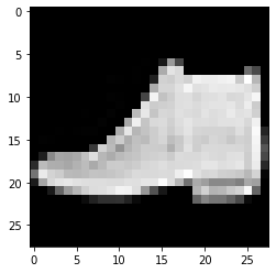
读入后，我们可以做一些数据可视化操作，主要是验证我们读入的数据是否正确

import matplotlib.pyplot as plt
image, label = next(iter(train_loader))
print(image.shape, label.shape)
plt.imshow(image[0][0], cmap="gray")

torch.Size([256, 1, 28, 28]) torch.Size([256])
<matplotlib.image.AxesImage at 0x1b39b49fcc8>

4.模型设计

# 使用CNN
class Net(nn.Module):
    def __init__(self):
        super(Net, self).__init__()
        self.conv = nn.Sequential(
            nn.Conv2d(1, 32, 5),
            nn.ReLU(),
            nn.MaxPool2d(2, stride=2),
            nn.Dropout(0.3),
            nn.Conv2d(32, 64, 5),
            nn.ReLU(),
            nn.MaxPool2d(2, stride=2),
            nn.Dropout(0.3)
        )
        self.fc = nn.Sequential(
            nn.Linear(64*4*4, 512),
            nn.ReLU(),
            nn.Linear(512, 10)
        )
        
    def forward(self, x):
        x = self.conv(x)
        x = x.view(-1, 64*4*4)
        x = self.fc(x)
        # x = nn.functional.normalize(x)
        return x

model = Net()
model = model.cuda()

5 设置损失函数和优化器

使用torch.nn模块自带的CrossEntropy损失。
PyTorch会自动把整数型的label转为one-hot型，用于计算CE loss
这里需要确保label是从0开始的，同时模型不加softmax层（使用logits计算）,这也说明了PyTorch训练中各个部分不是独立的，需要通盘考虑。

# 使用交叉熵损失函数
criterion = nn.CrossEntropyLoss()

# 使用Adam优化器
optimizer = optim.Adam(model.parameters(), lr=0.001)

6.训练与测试

各自封装成函数，方便后续调用
关注两者的主要区别：

模型状态设置
是否需要初始化优化器
是否需要将loss传回到网络
是否需要每步更新optimizer

此外，对于测试或验证过程，可以计算分类准确率。

训练：

def train(epoch):
    # 设置训练状态
    model.train()
    train_loss = 0
    # 循环读取DataLoader中的全部数据
    for data, label in train_loader:
        # 将数据放到GPU用于后续计算
        data, label = data.cuda(), label.cuda()
        # 将优化器的梯度清0
        optimizer.zero_grad()
        # 将数据输入给模型
        output = model(data)
        # 设置损失函数
        loss = criterion(output, label)
        # 将loss反向传播给网络
        loss.backward()
        # 使用优化器更新模型参数
        optimizer.step()
        # 累加训练损失
        train_loss += loss.item() * data.size(0)
    train_loss = train_loss/len(train_loader.dataset)
    print('Epoch: {} \tTraining Loss: {:.6f}'.format(epoch, train_loss))

验证：

def val(epoch): 
    # 设置验证状态
    model.eval()
    val_loss = 0
    gt_labels = []
    pred_labels = []
    # 不设置梯度
    with torch.no_grad():
        for data, label in test_loader:
            data, label = data.cuda(), label.cuda()
            output = model(data)
            preds = torch.argmax(output, 1)
            gt_labels.append(label.cpu().data.numpy())
            pred_labels.append(preds.cpu().data.numpy())
            loss = criterion(output, label)
            val_loss += loss.item()*data.size(0)
    # 计算验证集的平均损失
    val_loss = val_loss/len(test_loader.dataset)
    gt_labels, pred_labels = np.concatenate(gt_labels), np.concatenate(pred_labels)
    # 计算准确率
    acc = np.sum(gt_labels==pred_labels)/len(pred_labels)
    print('Epoch: {} \tValidation Loss: {:.6f}, Accuracy: {:6f}'.format(epoch, val_loss, acc))

for epoch in range(1, epochs+1):
    train(epoch)
    val(epoch)

Epoch: 1     Training Loss: 0.664049
Epoch: 1     Validation Loss: 0.421500, Accuracy: 0.852400
Epoch: 2     Training Loss: 0.417311
Epoch: 2     Validation Loss: 0.349790, Accuracy: 0.871200
Epoch: 3     Training Loss: 0.355448
Epoch: 3     Validation Loss: 0.318987, Accuracy: 0.879500
Epoch: 4     Training Loss: 0.323644
Epoch: 4     Validation Loss: 0.290521, Accuracy: 0.893800
Epoch: 5     Training Loss: 0.301900
Epoch: 5     Validation Loss: 0.266420, Accuracy: 0.901300
Epoch: 6     Training Loss: 0.286696
Epoch: 6     Validation Loss: 0.246448, Accuracy: 0.909700
Epoch: 7     Training Loss: 0.271441
Epoch: 7     Validation Loss: 0.241845, Accuracy: 0.911200
Epoch: 8     Training Loss: 0.260185
Epoch: 8     Validation Loss: 0.243311, Accuracy: 0.910800
Epoch: 9     Training Loss: 0.247986
Epoch: 9     Validation Loss: 0.225896, Accuracy: 0.916200
Epoch: 10     Training Loss: 0.240718
Epoch: 10     Validation Loss: 0.227848, Accuracy: 0.914700
Epoch: 11     Training Loss: 0.232358
Epoch: 11     Validation Loss: 0.220180, Accuracy: 0.917500
Epoch: 12     Training Loss: 0.223933
Epoch: 12     Validation Loss: 0.215308, Accuracy: 0.919400
Epoch: 13     Training Loss: 0.218354
Epoch: 13     Validation Loss: 0.211890, Accuracy: 0.919300
Epoch: 14     Training Loss: 0.210027
Epoch: 14     Validation Loss: 0.209707, Accuracy: 0.922700
Epoch: 15     Training Loss: 0.203024
Epoch: 15     Validation Loss: 0.208233, Accuracy: 0.925600
Epoch: 16     Training Loss: 0.196965
Epoch: 16     Validation Loss: 0.208209, Accuracy: 0.921900
Epoch: 17     Training Loss: 0.193155
Epoch: 17     Validation Loss: 0.200000, Accuracy: 0.926100
Epoch: 18     Training Loss: 0.184376
Epoch: 18     Validation Loss: 0.197259, Accuracy: 0.926200
Epoch: 19     Training Loss: 0.184272
Epoch: 19     Validation Loss: 0.200259, Accuracy: 0.926000
Epoch: 20     Training Loss: 0.172641
Epoch: 20     Validation Loss: 0.200177, Accuracy: 0.927100

7.模型保存

训练完成后，可以使用torch.save保存模型参数或者整个模型，也可以在训练过程中保存模型

save_path = "./FahionModel.pkl"
torch.save(model, save_path)

PyTorch学习笔记（五）：模型定义、修改、保存

一、PyTorch模型定义的方式

Module 类是 torch.nn 模块里提供的一个模型构造类 (nn.Module)，是所有神经⽹网络模块的基类，我们可以继承它来定义我们想要的模型；
PyTorch模型定义应包括两个主要部分：各个部分的初始化（_init_）；数据流向定义（forward）

基于nn.Module，可以通过Sequential，ModuleList和ModuleDict三种方式定义PyTorch模型。

1.Sequential

对应模块为nn.Sequential()。

当模型的前向计算为简单串联各个层的计算时， Sequential 类可以通过更加简单的方式定义模型。它可以接收一个子模块的有序字典(OrderedDict) 或者一系列子模块作为参数来逐一添加 Module 的实例，⽽模型的前向计算就是将这些实例按添加的顺序逐⼀计算。我们结合Sequential和定义方式加以理解：

class MySequential(nn.Module):
    from collections import OrderedDict
    def __init__(self, *args):
        super(MySequential, self).__init__()
        if len(args) == 1 and isinstance(args[0], OrderedDict): # 如果传入的是一个OrderedDict
            for key, module in args[0].items():
                self.add_module(key, module)  # add_module方法会将module添加进self._modules(一个OrderedDict)
        else:  # 传入的是一些Module
            for idx, module in enumerate(args):
                self.add_module(str(idx), module)
    def forward(self, input):
        # self._modules返回一个 OrderedDict，保证会按照成员添加时的顺序遍历成
        for module in self._modules.values():
            input = module(input)
        return input

下面来看下如何使用Sequential来定义模型。只需要将模型的层按序排列起来即可，根据层名的不同，排列的时候有两种方式：

直接排列

import torch.nn as nn
net = nn.Sequential(
        nn.Linear(784, 256),
        nn.ReLU(),
        nn.Linear(256, 10), 
        )
print(net)

Sequential(
  (0): Linear(in_features=784, out_features=256, bias=True)
  (1): ReLU()
  (2): Linear(in_features=256, out_features=10, bias=True)
)

OrderedDict：

import collections
import torch.nn as nn
net2 = nn.Sequential(collections.OrderedDict([
          ('fc1', nn.Linear(784, 256)),
          ('relu1', nn.ReLU()),
          ('fc2', nn.Linear(256, 10))
          ]))
print(net2)

Sequential(
  (fc1): Linear(in_features=784, out_features=256, bias=True)
  (relu1): ReLU()
  (fc2): Linear(in_features=256, out_features=10, bias=True)
)

可以看到，使用Sequential定义模型的好处在于简单、易读，同时使用Sequential定义的模型不需要再写forward，因为顺序已经定义好了。但使用Sequential也会使得模型定义丧失灵活性，比如需要在模型中间加入一个外部输入时就不适合用Sequential的方式实现。使用时需根据实际需求加以选择。

2.ModuleList

对应模块为nn.ModuleList()。

ModuleList 接收一个子模块（或层，需属于nn.Module类）的列表作为输入，然后也可以类似List那样进行append和extend操作。同时，子模块或层的权重也会自动添加到网络中来。

net = nn.ModuleList([nn.Linear(784, 256), nn.ReLU()])
net.append(nn.Linear(256, 10)) # # 类似List的append操作
print(net[-1])  # 类似List的索引访问
print(net)

Linear(in_features=256, out_features=10, bias=True)
ModuleList(
  (0): Linear(in_features=784, out_features=256, bias=True)
  (1): ReLU()
  (2): Linear(in_features=256, out_features=10, bias=True)
)

要特别注意的是，nn.ModuleList 并没有定义一个网络，它只是将不同的模块储存在一起。ModuleList中元素的先后顺序并不代表其在网络中的真实位置顺序，需要经过forward函数指定各个层的先后顺序后才算完成了模型的定义。具体实现时用for循环即可完成：

class model(nn.Module):
  def __init__(self, ...):
    self.modulelist = ...
    ...
    
  def forward(self, x):
    for layer in self.modulelist:
      x = layer(x)
    return x

3.ModuleDict

对应模块为nn.ModuleDict()。

ModuleDict和ModuleList的作用类似，只是ModuleDict能够更方便地为神经网络的层添加名称。

net = nn.ModuleDict({
    'linear': nn.Linear(784, 256),
    'act': nn.ReLU(),
})
net['output'] = nn.Linear(256, 10) # 添加
print(net['linear']) # 访问
print(net.output)
print(net)

Linear(in_features=784, out_features=256, bias=True)
Linear(in_features=256, out_features=10, bias=True)
ModuleDict(
  (act): ReLU()
  (linear): Linear(in_features=784, out_features=256, bias=True)
  (output): Linear(in_features=256, out_features=10, bias=True)
)

三种方法的比较总结

Sequential适用于快速验证结果，不需要同时写__init__和forward；
ModuleList和ModuleDict在某个完全相同的层需要重复出现多次时，非常方便实现，可以”一行顶多行“；
当我们需要之前层的信息的时候，比如 ResNets 中的残差计算，当前层的结果需要和之前层中的结果进行融合，一般使用 ModuleList/ModuleDict 比较方便。

二、利用模型块快速搭建复杂网络

模型搭建基本方法：

模型块分析
模型块实现
利用模型块组装模型

以U-Net模型为例，该模型为分割模型，通过残差连接结构解决了模型学习中的退化问题，使得神经网络的深度能够不断扩展。

模型块分析

每个子块内部的两次卷积DoubleConv
左侧模型块之间的下采样连接Down，通过Max pooling来实现
右侧模型块之间的上采样连接Up
输出层的处理OutConv
模型块之间的横向连接，输入和U-Net底部的连接等计算，这些单独的操作可以通过forward函数来实现

模型块实现

以U-net为例：

# 两次卷积 conv 3x3, ReLU
class DoubleConv(nn.Module):
    """(convolution => [BN] => ReLU) * 2"""
 
    def __init__(self, in_channels, out_channels, mid_channels=None):
        super().__init__()
        if not mid_channels:
            mid_channels = out_channels
        self.double_conv = nn.Sequential(
            nn.Conv2d(in_channels, mid_channels, kernel_size=3, padding=1, bias=False),
            nn.BatchNorm2d(mid_channels),
            nn.ReLU(inplace=True),
            nn.Conv2d(mid_channels, out_channels, kernel_size=3, padding=1, bias=False),
            nn.BatchNorm2d(out_channels),
            nn.ReLU(inplace=True)
        )
 
    def forward(self, x):
        return self.double_conv(x)
 
 
 
# 下采样 max pool 2x2
class Down(nn.Module):
    """Downscaling with maxpool then double conv"""
 
    def __init__(self, in_channels, out_channels):
        super().__init__()
        self.maxpool_conv = nn.Sequential(
            nn.MaxPool2d(2),
            DoubleConv(in_channels, out_channels)
        )
 
    def forward(self, x):
        return self.maxpool_conv(x)
# 上采样 up-conv 2x2
class Up(nn.Module):
    """Upscaling then double conv"""
 
    def __init__(self, in_channels, out_channels, bilinear=True):
        super().__init__()
 
        # if bilinear, use the normal convolutions to reduce the number of channels
        if bilinear:
            self.up = nn.Upsample(scale_factor=2, mode='bilinear', align_corners=True)
            self.conv = DoubleConv(in_channels, out_channels, in_channels // 2)
        else:
            self.up = nn.ConvTranspose2d(in_channels, in_channels // 2, kernel_size=2, stride=2)
            self.conv = DoubleConv(in_channels, out_channels)
 
    def forward(self, x1, x2):
        x1 = self.up(x1)
        # input is CHW
        diffY = x2.size()[2] - x1.size()[2]
        diffX = x2.size()[3] - x1.size()[3]
 
        x1 = F.pad(x1, [diffX // 2, diffX - diffX // 2,
                        diffY // 2, diffY - diffY // 2])
        x = torch.cat([x2, x1], dim=1)
 
# 输出 conv 1x1
class OutConv(nn.Module):
    def __init__(self, in_channels, out_channels):
        super(OutConv, self).__init__()
        self.conv = nn.Conv2d(in_channels, out_channels, kernel_size=1)
 
    def forward(self, x):
        return self.conv(x)

利用模型块组装U-net模型

class UNet(nn.Module):
    def __init__(self, n_channels, n_classes, bilinear=True):
        super(UNet, self).__init__()
        self.n_channels = n_channels
        self.n_classes = n_classes
        self.bilinear = bilinear
        
        self.inc = DoubleConv(n_channels, 64)
        self.down1 = Down(64, 128)
        self.down2 = Down(128, 256)
        self.down3 = Down(256, 512)
        factor = 2 if bilinear else 1
        self.down4 = Down(512, 1024 // factor)
        self.up1 = Up(1024, 512 // factor, bilinear)
        self.up2 = Up(512, 256 // factor, bilinear)
        self.up3 = Up(256, 128 // factor, bilinear)
        self.up4 = Up(128, 64, bilinear)
        self.outc = OutConv(64, n_classes)
    
    def forward(self, x):
        x1 = self.inc(x)
        x2 = self.down1(x1)
        x3 = self.down2(x2)
        x4 = self.down3(x3)
        x5 = self.down4(x4)
        x = self.up1(x5, x4)
        x = self.up2(x, x3)
        x = self.up3(x, x2)
        x = self.up4(x, x1)
        logits = self.outc(x)
        return logits

三、PyTorch修改模型

1.模型层

以pytorch中torchvision库预定义好的模型ResNet50为例，模型参数如下：

import torchvision.models as models
net = models.resnet50()
print(net)

ResNet(
  (conv1): Conv2d(3, 64, kernel_size=(7, 7), stride=(2, 2), padding=(3, 3), bias=False)
  (bn1): BatchNorm2d(64, eps=1e-05, momentum=0.1, affine=True, track_running_stats=True)
  (relu): ReLU(inplace=True)
  (maxpool): MaxPool2d(kernel_size=3, stride=2, padding=1, dilation=1, ceil_mode=False)
  (layer1): Sequential(
    (0): Bottleneck(
      (conv1): Conv2d(64, 64, kernel_size=(1, 1), stride=(1, 1), bias=False)
      (bn1): BatchNorm2d(64, eps=1e-05, momentum=0.1, affine=True, track_running_stats=True)
      (conv2): Conv2d(64, 64, kernel_size=(3, 3), stride=(1, 1), padding=(1, 1), bias=False)
      (bn2): BatchNorm2d(64, eps=1e-05, momentum=0.1, affine=True, track_running_stats=True)
      (conv3): Conv2d(64, 256, kernel_size=(1, 1), stride=(1, 1), bias=False)
      (bn3): BatchNorm2d(256, eps=1e-05, momentum=0.1, affine=True, track_running_stats=True)
      (relu): ReLU(inplace=True)
      (downsample): Sequential(
        (0): Conv2d(64, 256, kernel_size=(1, 1), stride=(1, 1), bias=False)
        (1): BatchNorm2d(256, eps=1e-05, momentum=0.1, affine=True, track_running_stats=True)
      )
    )
..............
  (avgpool): AdaptiveAvgPool2d(output_size=(1, 1))
  (fc): Linear(in_features=2048, out_features=1000, bias=True)
)

为了适配ImageNet预训练的权重，因此最后全连接层（fc）的输出节点数是1000。假设我们要用这个resnet模型去做一个10分类的问题，就应该修改模型的fc层，将其输出节点数替换为10。另外，我们觉得一层全连接层可能太少了，想再加一层。

可以做如下修改：

from collections import OrderedDict
classifier = nn.Sequential(OrderedDict([('fc1', nn.Linear(2048, 128)),
                          ('relu1', nn.ReLU()), 
                          ('dropout1',nn.Dropout(0.5)),
                          ('fc2', nn.Linear(128, 10)),
                          ('output', nn.Softmax(dim=1))
                          ]))
    
net.fc = classifier

这里的操作相当于将模型（net）最后名称为“fc”的层替换成了名称为“classifier”的结构，该结构是我们自己定义的。这里使用了Sequential+OrderedDict的模型定义方式，现在的模型就可以去做10分类任务了。

2.添加外部输入

有时候在模型训练中，除了已有模型的输入之外，还需要输入额外的信息。比如在CNN网络中，我们除了输入图像，还需要同时输入图像对应的其他信息，这时候就需要在已有的CNN网络中添加额外的输入变量。基本思路是：将原模型添加输入位置前的部分作为一个整体，同时在forward中定义好原模型不变的部分、添加的输入和后续层之间的连接关系，从而完成模型的修改。

我们以torchvision的resnet50模型为基础，任务还是10分类任务。不同点在于，我们希望利用已有的模型结构，在倒数第二层增加一个额外的输入变量add_variable来辅助预测。具体实现如下：

class Model(nn.Module):
    def __init__(self, net):
        super(Model, self).__init__()
        self.net = net
        self.relu = nn.ReLU()
        self.dropout = nn.Dropout(0.5)
        self.fc_add = nn.Linear(1001, 10, bias=True)
        self.output = nn.Softmax(dim=1)
        
    def forward(self, x, add_variable):
        x = self.net(x)
        x = torch.cat((self.dropout(self.relu(x)), add_variable.unsqueeze(1)),1)
        x = self.fc_add(x)
        x = self.output(x)
        return x

这里的实现要点是通过torch.cat实现了tensor的拼接。torchvision中的resnet50输出是一个1000维的tensor，我们通过修改forward函数（配套定义一些层），先将2048维的tensor通过激活函数层和dropout层，再和外部输入变量"add_variable"拼接，最后通过全连接层映射到指定的输出维度10。

另外这里对外部输入变量"add_variable"进行unsqueeze操作是为了和net输出的tensor保持维度一致，常用于add_variable是单一数值 (scalar) 的情况，此时add_variable的维度是 (batch_size, )，需要在第二维补充维数1，从而可以和tensor进行torch.cat操作。对于unsqueeze操作可以复习下2.1节的内容和配套代码 😃

之后对我们修改好的模型结构进行实例化，就可以使用了：

import torchvision.models as models
net = models.resnet50()
model = Model(net).cuda()

另外别忘了，训练中在输入数据的时候要给两个inputs：

outputs = model(inputs, add_var)

3.添加额外输出

有时候在模型训练中，除了模型最后的输出外，我们需要输出模型某一中间层的结果，以施加额外的监督，获得更好的中间层结果。基本的思路是修改模型定义中forward函数的return变量。

我们依然以resnet50做10分类任务为例，在已经定义好的模型结构上，同时输出1000维的倒数第二层和10维的最后一层结果。具体实现如下：

class Model(nn.Module):
    def __init__(self, net):
        super(Model, self).__init__()
        self.net = net
        self.relu = nn.ReLU()
        self.dropout = nn.Dropout(0.5)
        self.fc1 = nn.Linear(1000, 10, bias=True)
        self.output = nn.Softmax(dim=1)
        
    def forward(self, x, add_variable):
        x1000 = self.net(x)
        x10 = self.dropout(self.relu(x1000))
        x10 = self.fc1(x10)
        x10 = self.output(x10)
        return x10, x1000

之后对我们修改好的模型结构进行实例化，就可以使用了：

import torchvision.models as models
net = models.resnet50()
model = Model(net).cuda()
#另外别忘了，训练中在输入数据后会有两个outputs：
 
out10, out1000 = model(inputs, add_var)

四、PyTorch模型保存与读取

1.模型存储格式

PyTorch存储模型主要采用pkl，pt，pth三种格式。就使用层面来说没有区别，这里不做具体的讨论。本节最后的参考内容中列出了查阅到的一些资料，感兴趣的读者可以进一步研究，欢迎留言讨论。

3.模型存储内容

一个PyTorch模型主要包含两个部分：模型结构和权重。其中模型是继承nn.Module的类，权重的数据结构是一个字典（key是层名，value是权重向量）。存储也由此分为两种形式：存储整个模型（包括结构和权重），和只存储模型权重。

from torchvision import models
model = models.resnet152(pretrained=True)
 
# 保存整个模型
torch.save(model, save_dir)
# 保存模型权重
torch.save(model.state_dict, save_dir)

对于PyTorch而言，pt, pth和pkl三种数据格式均支持模型权重和整个模型存储，使用上没有差别。

保存+读取整个模型

torch.save(model, save_dir)
loaded_model = torch.load(save_dir)
loaded_model.cuda()

保存+读取模型权重

torch.save(model.state_dict(), save_dir)
loaded_dict = torch.load(save_dir)
loaded_model = models.resnet152()   #注意这里需要对模型结构有定义
loaded_model.state_dict = loaded_dict
loaded_model.cuda()

模型保存文章推荐：阿里云登录 - 欢迎登录阿里云，安全稳定的云计算服务平台

PyTorch学习笔记（六）：PyTorch进阶训练技巧

import torch
import torch.nn as nn
import torch.nn.functional as F

1 自定义损失函数

以函数方式定义：通过输出值和目标值进行计算，返回损失值
以类方式定义：通过继承nn.Module，将其当做神经网络的一层来看待

以DiceLoss损失函数为例，定义如下：

DSC = \frac{2|X∩Y|}{|X|+|Y|}DSC=∣X∣+∣Y∣2∣X∩Y∣

class DiceLoss(nn.Module):
    def __init__(self, weight=None, size_average=True):
        super(DiceLoss,self).__init__()
        
    def forward(self, inputs, targets, smooth=1):
        inputs = F.sigmoid(inputs)       
        inputs = inputs.view(-1)
        targets = targets.view(-1)
        intersection = (inputs * targets).sum()                   
        dice = (2.*intersection + smooth)/(inputs.sum() + targets.sum() + smooth)  
        return 1 - dice

2 动态调整学习率

Scheduler：学习率衰减策略，解决学习率选择的问题，用于提高精度
PyTorch Scheduler策略：
- lr_scheduler.LambdaLR
- lr_scheduler.MultiplicativeLR
- lr_scheduler.StepLR
- lr_scheduler.MultiStepLR
- lr_scheduler.ExponentialLR
- lr_scheduler.CosineAnnealingLR
- lr_scheduler.ReduceLROnPlateau
- lr_scheduler.CyclicLR
- lr_scheduler.OneCycleLR
- lr_scheduler.CosineAnnealingWarmRestarts
使用说明：需要将scheduler.step()放在optimizer.step()后面
自定义Scheduler：通过自定义函数对学习率进行修改

3 模型微调

概念：找到一个同类已训练好的模型，调整模型参数，使用数据进行训练。
模型微调的流程
1. 在源数据集上预训练一个神经网络模型，即源模型
2. 创建一个新的神经网络模型，即目标模型，该模型复制了源模型上除输出层外的所有模型设计和参数
3. 给目标模型添加一个输出大小为目标数据集类别个数的输出层，并随机初始化改成的模型参数
4. 使用目标数据集训练目标模型

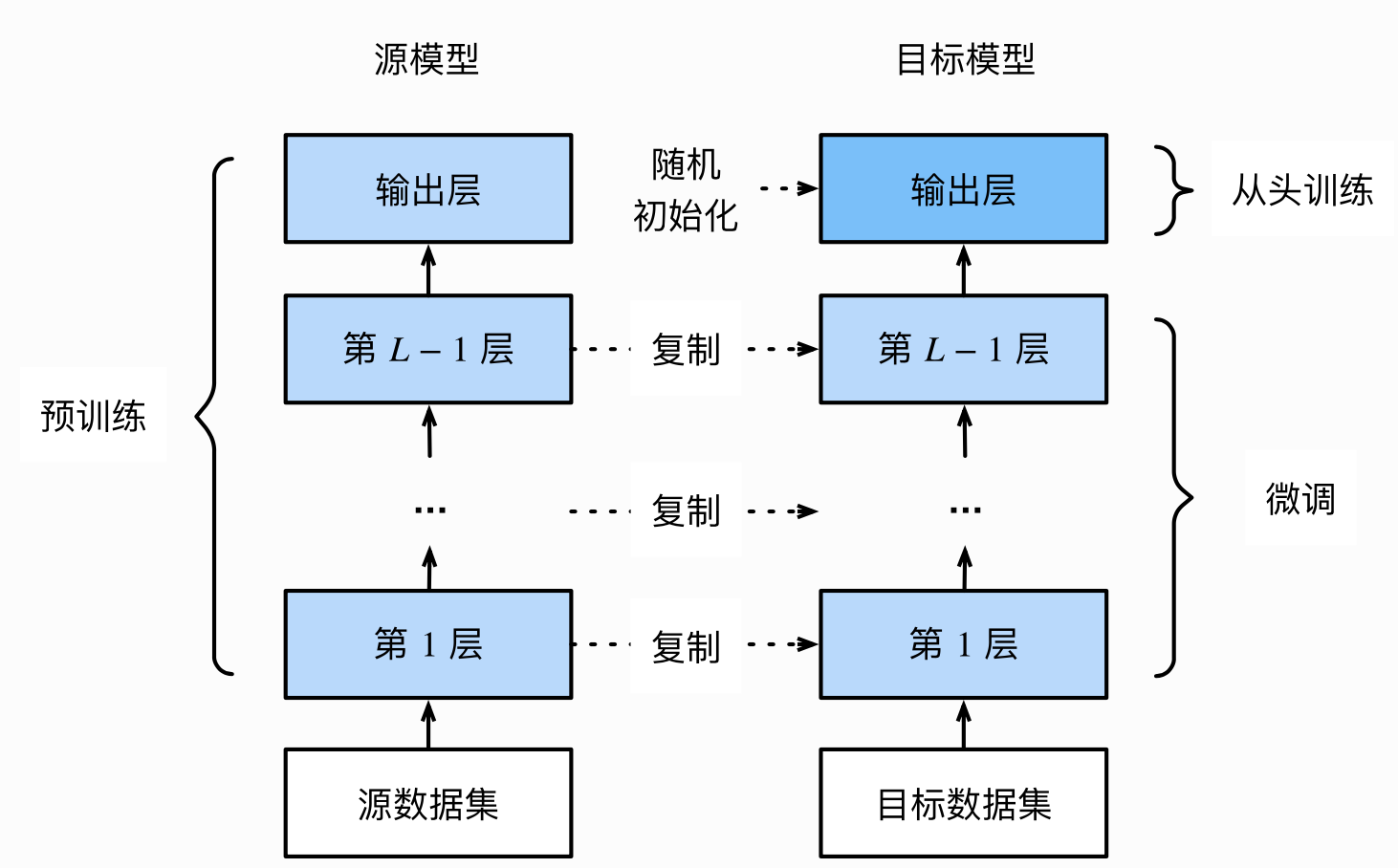
使用已有模型结构：通过传入pretrained参数，决定是否使用预训练好的权重

训练特定层：使用requires_grad=False冻结部分网络层，只计算新初始化的层的梯度

def set_parameter_requires_grad(model, feature_extracting):
if feature_extracting:
    for param in model.parameters():
        param.requires_grad = False

import torchvision.models as models

冻结参数的梯度

feature_extract = True
model = models.resnet50(pretrained=True)
set_parameter_requires_grad(model, feature_extract)

修改模型

num_ftrs = model.fc.in_features
model.fc = nn.Linear(in_features=512, out_features=4, bias=True)

model.fc

Linear(in_features=512, out_features=4, bias=True)
```

注：在训练过程中，model仍会回传梯度，但是参数更新只会发生在`fc`层。

4 半精度训练

半精度优势：减少显存占用，提高GPU同时加载的数据量
设置半精度训练：
1. 导入torch.cuda.amp的autocast包
2. 在模型定义中的forward函数上，设置autocast装饰器
3. 在训练过程中，在数据输入模型之后，添加with autocast()
适用范围：适用于数据的size较大的数据集（比如3D图像、视频等）

5 总结

自定义损失函数可以通过二种方式：函数方式和类方式，建议全程使用PyTorch提供的张量计算方法。
通过使用PyTorch中的scheduler动态调整学习率，也支持自定义scheduler
模型微调主要使用已有的预训练模型，调整其中的参数构建目标模型，在目标数据集上训练模型。
半精度训练主要适用于数据的size较大的数据集（比如3D图像、视频等）。

PyTorch学习笔记（七）：PyTorch可视化_

1 可视化网络结构

打印模型基础信息：使用print()函数，只能打印出基础构件的信息，不能显示每一层的shape和对应参数量的大小

 import torchvision.models as models
 
 model = models.resnet18()

print(model)

ResNet(
  (conv1): Conv2d(3, 64, kernel_size=(7, 7), stride=(2, 2), padding=(3, 3), bias=False)
  (bn1): BatchNorm2d(64, eps=1e-05, momentum=0.1, affine=True, track_running_stats=True)
  (relu): ReLU(inplace=True)
  (maxpool): MaxPool2d(kernel_size=3, stride=2, padding=1, dilation=1, ceil_mode=False)
  (layer1): Sequential(
    (0): BasicBlock(
      (conv1): Conv2d(64, 64, kernel_size=(3, 3), stride=(1, 1), padding=(1, 1), bias=False)
      (bn1): BatchNorm2d(64, eps=1e-05, momentum=0.1, affine=True, track_running_stats=True)
      (relu): ReLU(inplace=True)
      (conv2): Conv2d(64, 64, kernel_size=(3, 3), stride=(1, 1), padding=(1, 1), bias=False)
      (bn2): BatchNorm2d(64, eps=1e-05, momentum=0.1, affine=True, track_running_stats=True)
    )
    (1): BasicBlock(
      (conv1): Conv2d(64, 64, kernel_size=(3, 3), stride=(1, 1), padding=(1, 1), bias=False)
      (bn1): BatchNorm2d(64, eps=1e-05, momentum=0.1, affine=True, track_running_stats=True)
      (relu): ReLU(inplace=True)
      (conv2): Conv2d(64, 64, kernel_size=(3, 3), stride=(1, 1), padding=(1, 1), bias=False)
      (bn2): BatchNorm2d(64, eps=1e-05, momentum=0.1, affine=True, track_running_stats=True)
    )
  )
  (layer2): Sequential(
    (0): BasicBlock(
      (conv1): Conv2d(64, 128, kernel_size=(3, 3), stride=(2, 2), padding=(1, 1), bias=False)
      (bn1): BatchNorm2d(128, eps=1e-05, momentum=0.1, affine=True, track_running_stats=True)
      (relu): ReLU(inplace=True)
      (conv2): Conv2d(128, 128, kernel_size=(3, 3), stride=(1, 1), padding=(1, 1), bias=False)
      (bn2): BatchNorm2d(128, eps=1e-05, momentum=0.1, affine=True, track_running_stats=True)
      (downsample): Sequential(
        (0): Conv2d(64, 128, kernel_size=(1, 1), stride=(2, 2), bias=False)
        (1): BatchNorm2d(128, eps=1e-05, momentum=0.1, affine=True, track_running_stats=True)
      )
    )
    (1): BasicBlock(
      (conv1): Conv2d(128, 128, kernel_size=(3, 3), stride=(1, 1), padding=(1, 1), bias=False)
      (bn1): BatchNorm2d(128, eps=1e-05, momentum=0.1, affine=True, track_running_stats=True)
      (relu): ReLU(inplace=True)
      (conv2): Conv2d(128, 128, kernel_size=(3, 3), stride=(1, 1), padding=(1, 1), bias=False)
      (bn2): BatchNorm2d(128, eps=1e-05, momentum=0.1, affine=True, track_running_stats=True)
    )
  )
  (layer3): Sequential(
    (0): BasicBlock(
      (conv1): Conv2d(128, 256, kernel_size=(3, 3), stride=(2, 2), padding=(1, 1), bias=False)
      (bn1): BatchNorm2d(256, eps=1e-05, momentum=0.1, affine=True, track_running_stats=True)
      (relu): ReLU(inplace=True)
      (conv2): Conv2d(256, 256, kernel_size=(3, 3), stride=(1, 1), padding=(1, 1), bias=False)
      (bn2): BatchNorm2d(256, eps=1e-05, momentum=0.1, affine=True, track_running_stats=True)
      (downsample): Sequential(
        (0): Conv2d(128, 256, kernel_size=(1, 1), stride=(2, 2), bias=False)
        (1): BatchNorm2d(256, eps=1e-05, momentum=0.1, affine=True, track_running_stats=True)
      )
    )
    (1): BasicBlock(
      (conv1): Conv2d(256, 256, kernel_size=(3, 3), stride=(1, 1), padding=(1, 1), bias=False)
      (bn1): BatchNorm2d(256, eps=1e-05, momentum=0.1, affine=True, track_running_stats=True)
      (relu): ReLU(inplace=True)
      (conv2): Conv2d(256, 256, kernel_size=(3, 3), stride=(1, 1), padding=(1, 1), bias=False)
      (bn2): BatchNorm2d(256, eps=1e-05, momentum=0.1, affine=True, track_running_stats=True)
    )
  )
  (layer4): Sequential(
    (0): BasicBlock(
      (conv1): Conv2d(256, 512, kernel_size=(3, 3), stride=(2, 2), padding=(1, 1), bias=False)
      (bn1): BatchNorm2d(512, eps=1e-05, momentum=0.1, affine=True, track_running_stats=True)
      (relu): ReLU(inplace=True)
      (conv2): Conv2d(512, 512, kernel_size=(3, 3), stride=(1, 1), padding=(1, 1), bias=False)
      (bn2): BatchNorm2d(512, eps=1e-05, momentum=0.1, affine=True, track_running_stats=True)
      (downsample): Sequential(
        (0): Conv2d(256, 512, kernel_size=(1, 1), stride=(2, 2), bias=False)
        (1): BatchNorm2d(512, eps=1e-05, momentum=0.1, affine=True, track_running_stats=True)
      )
    )
    (1): BasicBlock(
      (conv1): Conv2d(512, 512, kernel_size=(3, 3), stride=(1, 1), padding=(1, 1), bias=False)
      (bn1): BatchNorm2d(512, eps=1e-05, momentum=0.1, affine=True, track_running_stats=True)
      (relu): ReLU(inplace=True)
      (conv2): Conv2d(512, 512, kernel_size=(3, 3), stride=(1, 1), padding=(1, 1), bias=False)
      (bn2): BatchNorm2d(512, eps=1e-05, momentum=0.1, affine=True, track_running_stats=True)
    )
  )
  (avgpool): AdaptiveAvgPool2d(output_size=(1, 1))
  (fc): Linear(in_features=512, out_features=1000, bias=True)
)

可视化网络结构：使用torchinfo库进行模型网络的结构输出，可以得到更加详细的信息，包括模块信息（每一层的类型、输出shape和参数量）、模型整体的参数量、模型大小、一次前向或者反向传播需要的内存大小等

import torchvision.models as models
from torchinfo import summary
 
resnet18 = models.resnet18() # 实例化模型
# 其中batch_size为1，图片的通道数为3，图片的高宽为224
summary(model, (1, 3, 224, 224))

==========================================================================================
Layer (type:depth-idx)                   Output Shape              Param #
==========================================================================================
ResNet                                   --                        --
├─Conv2d: 1-1                            [1, 64, 112, 112]         9,408
├─BatchNorm2d: 1-2                       [1, 64, 112, 112]         128
├─ReLU: 1-3                              [1, 64, 112, 112]         --
├─MaxPool2d: 1-4                         [1, 64, 56, 56]           --
├─Sequential: 1-5                        [1, 64, 56, 56]           --
│    └─BasicBlock: 2-1                   [1, 64, 56, 56]           --
│    │    └─Conv2d: 3-1                  [1, 64, 56, 56]           36,864
│    │    └─BatchNorm2d: 3-2             [1, 64, 56, 56]           128
│    │    └─ReLU: 3-3                    [1, 64, 56, 56]           --
│    │    └─Conv2d: 3-4                  [1, 64, 56, 56]           36,864
│    │    └─BatchNorm2d: 3-5             [1, 64, 56, 56]           128
│    │    └─ReLU: 3-6                    [1, 64, 56, 56]           --
│    └─BasicBlock: 2-2                   [1, 64, 56, 56]           --
│    │    └─Conv2d: 3-7                  [1, 64, 56, 56]           36,864
│    │    └─BatchNorm2d: 3-8             [1, 64, 56, 56]           128
│    │    └─ReLU: 3-9                    [1, 64, 56, 56]           --
│    │    └─Conv2d: 3-10                 [1, 64, 56, 56]           36,864
│    │    └─BatchNorm2d: 3-11            [1, 64, 56, 56]           128
│    │    └─ReLU: 3-12                   [1, 64, 56, 56]           --
├─Sequential: 1-6                        [1, 128, 28, 28]          --
│    └─BasicBlock: 2-3                   [1, 128, 28, 28]          --
│    │    └─Conv2d: 3-13                 [1, 128, 28, 28]          73,728
│    │    └─BatchNorm2d: 3-14            [1, 128, 28, 28]          256
│    │    └─ReLU: 3-15                   [1, 128, 28, 28]          --
│    │    └─Conv2d: 3-16                 [1, 128, 28, 28]          147,456
│    │    └─BatchNorm2d: 3-17            [1, 128, 28, 28]          256
│    │    └─Sequential: 3-18             [1, 128, 28, 28]          8,448
│    │    └─ReLU: 3-19                   [1, 128, 28, 28]          --
│    └─BasicBlock: 2-4                   [1, 128, 28, 28]          --
│    │    └─Conv2d: 3-20                 [1, 128, 28, 28]          147,456
│    │    └─BatchNorm2d: 3-21            [1, 128, 28, 28]          256
│    │    └─ReLU: 3-22                   [1, 128, 28, 28]          --
│    │    └─Conv2d: 3-23                 [1, 128, 28, 28]          147,456
│    │    └─BatchNorm2d: 3-24            [1, 128, 28, 28]          256
│    │    └─ReLU: 3-25                   [1, 128, 28, 28]          --
├─Sequential: 1-7                        [1, 256, 14, 14]          --
│    └─BasicBlock: 2-5                   [1, 256, 14, 14]          --
│    │    └─Conv2d: 3-26                 [1, 256, 14, 14]          294,912
│    │    └─BatchNorm2d: 3-27            [1, 256, 14, 14]          512
│    │    └─ReLU: 3-28                   [1, 256, 14, 14]          --
│    │    └─Conv2d: 3-29                 [1, 256, 14, 14]          589,824
│    │    └─BatchNorm2d: 3-30            [1, 256, 14, 14]          512
│    │    └─Sequential: 3-31             [1, 256, 14, 14]          33,280
│    │    └─ReLU: 3-32                   [1, 256, 14, 14]          --
│    └─BasicBlock: 2-6                   [1, 256, 14, 14]          --
│    │    └─Conv2d: 3-33                 [1, 256, 14, 14]          589,824
│    │    └─BatchNorm2d: 3-34            [1, 256, 14, 14]          512
│    │    └─ReLU: 3-35                   [1, 256, 14, 14]          --
│    │    └─Conv2d: 3-36                 [1, 256, 14, 14]          589,824
│    │    └─BatchNorm2d: 3-37            [1, 256, 14, 14]          512
│    │    └─ReLU: 3-38                   [1, 256, 14, 14]          --
├─Sequential: 1-8                        [1, 512, 7, 7]            --
│    └─BasicBlock: 2-7                   [1, 512, 7, 7]            --
│    │    └─Conv2d: 3-39                 [1, 512, 7, 7]            1,179,648
│    │    └─BatchNorm2d: 3-40            [1, 512, 7, 7]            1,024
│    │    └─ReLU: 3-41                   [1, 512, 7, 7]            --
│    │    └─Conv2d: 3-42                 [1, 512, 7, 7]            2,359,296
│    │    └─BatchNorm2d: 3-43            [1, 512, 7, 7]            1,024
│    │    └─Sequential: 3-44             [1, 512, 7, 7]            132,096
│    │    └─ReLU: 3-45                   [1, 512, 7, 7]            --
│    └─BasicBlock: 2-8                   [1, 512, 7, 7]            --
│    │    └─Conv2d: 3-46                 [1, 512, 7, 7]            2,359,296
│    │    └─BatchNorm2d: 3-47            [1, 512, 7, 7]            1,024
│    │    └─ReLU: 3-48                   [1, 512, 7, 7]            --
│    │    └─Conv2d: 3-49                 [1, 512, 7, 7]            2,359,296
│    │    └─BatchNorm2d: 3-50            [1, 512, 7, 7]            1,024
│    │    └─ReLU: 3-51                   [1, 512, 7, 7]            --
├─AdaptiveAvgPool2d: 1-9                 [1, 512, 1, 1]            --
├─Linear: 1-10                           [1, 1000]                 513,000
==========================================================================================
Total params: 11,689,512
Trainable params: 11,689,512
Non-trainable params: 0
Total mult-adds (G): 1.81
==========================================================================================
Input size (MB): 0.60
Forward/backward pass size (MB): 39.75
Params size (MB): 46.76
Estimated Total Size (MB): 87.11
==========================================================================================
Copy to clipboardErrorCopied

2 CNN可视化

CNN卷积核可视化

model = models.vgg11(pretrained=True)
dict(model.features.named_children())

{'0': Conv2d(3, 64, kernel_size=(3, 3), stride=(1, 1), padding=(1, 1)),
 '1': ReLU(inplace=True),
 '2': MaxPool2d(kernel_size=2, stride=2, padding=0, dilation=1, ceil_mode=False),
 '3': Conv2d(64, 128, kernel_size=(3, 3), stride=(1, 1), padding=(1, 1)),
 '4': ReLU(inplace=True),
 '5': MaxPool2d(kernel_size=2, stride=2, padding=0, dilation=1, ceil_mode=False),
 '6': Conv2d(128, 256, kernel_size=(3, 3), stride=(1, 1), padding=(1, 1)),
 '7': ReLU(inplace=True),
 '8': Conv2d(256, 256, kernel_size=(3, 3), stride=(1, 1), padding=(1, 1)),
 '9': ReLU(inplace=True),
 '10': MaxPool2d(kernel_size=2, stride=2, padding=0, dilation=1, ceil_mode=False),
 '11': Conv2d(256, 512, kernel_size=(3, 3), stride=(1, 1), padding=(1, 1)),
 '12': ReLU(inplace=True),
 '13': Conv2d(512, 512, kernel_size=(3, 3), stride=(1, 1), padding=(1, 1)),
 '14': ReLU(inplace=True),
 '15': MaxPool2d(kernel_size=2, stride=2, padding=0, dilation=1, ceil_mode=False),
 '16': Conv2d(512, 512, kernel_size=(3, 3), stride=(1, 1), padding=(1, 1)),
 '17': ReLU(inplace=True),
 '18': Conv2d(512, 512, kernel_size=(3, 3), stride=(1, 1), padding=(1, 1)),
 '19': ReLU(inplace=True),
 '20': MaxPool2d(kernel_size=2, stride=2, padding=0, dilation=1, ceil_mode=False)}

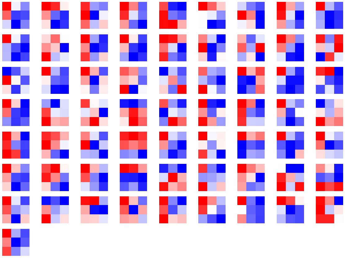
import matplotlib.pyplot as plt
 
conv1 = dict(model.features.named_children())['3']
# 得到第3层的卷积层参数
kernel_set = conv1.weight.detach()
num = len(conv1.weight.detach())
print(kernel_set.shape)
# 该代码仅可视化其中一个维度的卷积核，第3层的卷积核有128*64个
for i in range(0, 1):
    i_kernel = kernel_set[i]
    plt.figure(figsize=(20, 17))
    if (len(i_kernel)) > 1:
        for idx, filer in enumerate(i_kernel):
            plt.subplot(9, 9, idx+1) 
            plt.axis('off')
            plt.imshow(filer[ :, :].detach(),cmap='bwr')

torch.Size([128, 64, 3, 3])

CNN特征图可视化：使用PyTorch提供的hook结构，得到网络在前向传播过程中的特征图。
CNN class activation map可视化：用于在CNN可视化场景下，判断图像中哪些像素点对预测结果是重要的，可使用grad-cam库进行操作
使用FlashTorch快速实现CNDD可视化：可以使用flashtorch库，可视化梯度和卷积核

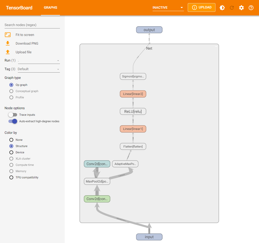
3 使用TensorBoard可视化训练过程

可视化基本逻辑：TensorBoard记录模型每一层的feature map、权重和训练loss等，并保存在用户指定的文件夹中，通过网页形式进行可视化展示
模型结构可视化：使用add_graph方法，在TensorBoard下展示模型结构

 import torch.nn as nn
 
class Net(nn.Module):
    def __init__(self):
        super(Net, self).__init__()
        self.conv1 = nn.Conv2d(in_channels=3,out_channels=32,kernel_size = 3)
        self.pool = nn.MaxPool2d(kernel_size = 2,stride = 2)
        self.conv2 = nn.Conv2d(in_channels=32,out_channels=64,kernel_size = 5)
        self.adaptive_pool = nn.AdaptiveMaxPool2d((1,1))
        self.flatten = nn.Flatten()
        self.linear1 = nn.Linear(64,32)
        self.relu = nn.ReLU()
        self.linear2 = nn.Linear(32,1)
        self.sigmoid = nn.Sigmoid()
 
    def forward(self,x):
        x = self.conv1(x)
        x = self.pool(x)
        x = self.conv2(x)
        x = self.pool(x)
        x = self.adaptive_pool(x)
        x = self.flatten(x)
        x = self.linear1(x)
        x = self.relu(x)
        x = self.linear2(x)
        y = self.sigmoid(x)
        return y

model = Net()
print(model)


Net(
  (conv1): Conv2d(3, 32, kernel_size=(3, 3), stride=(1, 1))
  (pool): MaxPool2d(kernel_size=2, stride=2, padding=0, dilation=1, ceil_mode=False)
  (conv2): Conv2d(32, 64, kernel_size=(5, 5), stride=(1, 1))
  (adaptive_pool): AdaptiveMaxPool2d(output_size=(1, 1))
  (flatten): Flatten(start_dim=1, end_dim=-1)
  (linear1): Linear(in_features=64, out_features=32, bias=True)
  (relu): ReLU()
  (linear2): Linear(in_features=32, out_features=1, bias=True)
  (sigmoid): Sigmoid()
)

from torch.utils.tensorboard import SummaryWriter
 
writer = SummaryWriter('./runs')
writer.add_graph(model, input_to_model = torch.rand(1, 3, 224, 224))
writer.close()

在当前目录下，执行tensorboard --logdir=./runs命令，打开TensorBoard可视化页面，看到模型网络结构。

图像可视化：
- 对于单张图片的显示使用add_image
- 对于多张图片的显示使用add_images
- 有时需要使用torchvision.utils.make_grid将多张图片拼成一张图片后，用writer.add_image显示
连续变量可视化：使用add_scalar方法，对连续变量（或时序变量）的变化过程进行可视化展示

for i in range(500):
    x = i
    y = x ** 2
    writer.add_scalar("x", x, i) #日志中记录x在第step i 的值
    writer.add_scalar("y", y, i) #日志中记录y在第step i 的值
writer.close()
Copy to clipboardErrorCopied

参数分布可视化：使用add_histogram方法，对参数（或变量）的分布进行可视化展示

import numpy as np
 
# 创建正态分布的张量模拟参数矩阵
def norm(mean, std):
    t = std * torch.randn((100, 20)) + mean
    return t
 
for step, mean in enumerate(range(-10, 10, 1)):
    w = norm(mean, 1)
    writer.add_histogram("w", w, step)
    writer.flush()
writer.close()
Copy to clipboardErrorCopied

4 总结

本次任务，主要介绍了PyTorch可视化，包括可视化网络结构、CNN卷积层可视化和使用TensorBoard可视化训练过程。

使用torchinfo库，可视化模型网络结构，展示模块信息（每一层的类型、输出shape和参数量）、模型整体的参数量、模型大小、一次前向或者反向传播需要的内存大小等。
使用grad-cam库，可视化重要像素点，能够快速确定重要区域，进行可解释性分析或模型优化改进。
通过TensorBoard工具，调用相关方法创建训练记录，可视化模型结构、图像、连续变量和参数分布等。

PyTorch学习笔记（八）：PyTorch生态简介

一、 torchvision（图像）

1.torchvision.datasets：

计算机视觉领域常见的数据集，包括CIFAR、EMNIST、Fashion-MNIST等

torchvision.datasets主要包含了一些我们在计算机视觉中常见的数据集，在0.10.0版本的torchvision下，有以下的数据集：

Caltech	CelebA	CIFAR	Cityscapes
EMNIST	FakeData	Fashion-MNIST	Flickr
ImageNet	Kinetics-400	KITTI	KMNIST
PhotoTour	Places365	QMNIST	SBD
SEMEION	STL10	SVHN	UCF101
VOC	WIDERFace

2.torchvision.transforms：

数据预处理方法，可以进行图片数据的放大、缩小、水平或垂直翻转等

from torchvision import transforms
data_transform = transforms.Compose([
    transforms.ToPILImage(),   # 这一步取决于后续的数据读取方式，如果使用内置数据集则不需要
    transforms.Resize(image_size),
    transforms.ToTensor()
])

3.torchvision.models：

预训练模型，包括图像分类、语义分割、物体检测、实例分割、人体关键点检测、视频分类等模型

为了提高训练效率，减少不必要的重复劳动，PyTorch官方也提供了一些预训练好的模型供我们使用，可以点击这里进行查看现在有哪些预训练模型，下面我们将对如何使用这些模型进行详细介绍。此处我们以torchvision0.10.0 为例，如果希望获取更多的预训练模型，可以使用使用pretrained-models.pytorch仓库。现有预训练好的模型可以分为以下几类：

Classification

在图像分类里面，PyTorch官方提供了以下模型，并正在不断增多。

AlexNet	VGG	ResNet	SqueezeNet
DenseNet	Inception v3	GoogLeNet	ShuffleNet v2
MobileNetV2	MobileNetV3	ResNext	Wide ResNet
MNASNet	EfficientNet	RegNet	持续更新

这些模型是在ImageNet-1k进行预训练好的，具体的使用我们会在后面进行介绍。除此之外，我们也可以点击这里去查看这些模型在ImageNet-1k的准确率。

Semantic Segmentation

语义分割的预训练模型是在COCO train2017的子集上进行训练的，提供了20个类别，包括background, aeroplane, bicycle, bird, boat, bottle, bus, car, cat, chair, cow, diningtable, dog, horse, motorbike, person, pottedplant, sheep, sofa,train, tvmonitor。

FCN ResNet50	FCN ResNet101	DeepLabV3 ResNet50	DeepLabV3 ResNet101
LR-ASPP MobileNetV3-Large	DeepLabV3 MobileNetV3-Large	未完待续

具体我们可以点击这里进行查看预训练的模型的mean IOU和global pixelwise acc

Object Detection，instance Segmentation and Keypoint Detection

物体检测，实例分割和人体关键点检测的模型我们同样是在COCO train2017进行训练的，在下方我们提供了实例分割的类别和人体关键点检测类别：

COCO_INSTANCE_CATEGORY_NAMES = [
‘background’, ‘person’, ‘bicycle’, ‘car’, ‘motorcycle’, ‘airplane’, ‘bus’,‘train’, ‘truck’, ‘boat’, ‘traffic light’, ‘fire hydrant’, ‘N/A’, ‘stop sign’, ‘parking meter’, ‘bench’, ‘bird’, ‘cat’, ‘dog’, ‘horse’, ‘sheep’, ‘cow’, ‘elephant’, ‘bear’, ‘zebra’, ‘giraffe’, ‘N/A’, ‘backpack’, ‘umbrella’, ‘N/A’, ‘N/A’,‘handbag’, ‘tie’, ‘suitcase’, ‘frisbee’, ‘skis’, ‘snowboard’, ‘sports ball’,‘kite’, ‘baseball bat’, ‘baseball glove’, ‘skateboard’, ‘surfboard’, ‘tennis racket’,‘bottle’, ‘N/A’, ‘wine glass’, ‘cup’, ‘fork’, ‘knife’, ‘spoon’, ‘bowl’,‘banana’, ‘apple’, ‘sandwich’, ‘orange’, ‘broccoli’, ‘carrot’, ‘hot dog’, ‘pizza’,‘donut’, ‘cake’, ‘chair’, ‘couch’, ‘potted plant’, ‘bed’, ‘N/A’, ‘dining table’,‘N/A’, ‘N/A’, ‘toilet’, ‘N/A’, ‘tv’, ‘laptop’, ‘mouse’, ‘remote’, ‘keyboard’, ‘cell phone’,‘microwave’, ‘oven’, ‘toaster’, ‘sink’, ‘refrigerator’, ‘N/A’, ‘book’,‘clock’, ‘vase’, ‘scissors’, ‘teddy bear’, ‘hair drier’, ‘toothbrush’]
COCO_PERSON_KEYPOINT_NAMES =[‘nose’,‘left_eye’,‘right_eye’,‘left_ear’,‘right_ear’,‘left_shoulder’,‘right_shoulder’,‘left_elbow’,‘right_elbow’,‘left_wrist’,‘right_wrist’,‘left_hip’,‘right_hip’,‘left_knee’,‘right_knee’,‘left_ankle’,‘right_ankle’]

Faster R-CNN	Mask R-CNN	RetinaNet	SSDlite
SSD	未完待续

同样的，我们可以点击这里查看这些模型在COCO train 2017上的box AP,keypoint AP,mask AP

Video classification

视频分类模型是在 Kinetics-400上进行预训练的

ResNet 3D 18	ResNet MC 18	ResNet (2+1) D
未完待续

同样我们也可以点击这里查看这些模型的。

4.torchvision.io：

视频、图片和文件的IO操作，包括读取、写入、编解码处理等

5.torchvision.ops：

计算机视觉的特定操作，包括但不仅限于NMS，RoIAlign（MASK R-CNN中应用的一种方法），RoIPool（Fast R-CNN中用到的一种方法）

6.torchvision.utils：

图片拼接、可视化检测和分割等操作

torchvision.utils 为我们提供了一些可视化的方法，可以帮助我们将若干张图片拼接在一起、可视化检测和分割的效果。具体方法可以点击这里进行查看。

总的来说，torchvision的出现帮助我们解决了常见的计算机视觉中一些重复且耗时的工作，并在数据集的获取、数据增强、模型预训练等方面大大降低了我们的工作难度，可以让我们更加快速上手一些计算机视觉任务。

2 PyTorchVideo（视频）

简介：PyTorchVideo是一个专注于视频理解工作的深度学习库，提供加速视频理解研究所需的可重用、模块化和高效的组件，使用PyTorch开发，支持不同的深度学习视频组件，如视频模型、视频数据集和视频特定转换。
特点：基于PyTorch，提供Model Zoo，支持数据预处理和常见数据，采用模块化设计，支持多模态，优化移动端部署
使用方式：TochHub、PySlowFast、PyTorch Lightning

3 torchtext（文本）

torchtext的主要组成部分

torchtext可以方便的对文本进行预处理，例如截断补长、构建词表等。torchtext主要包含了以下的主要组成部分：

数据处理工具 torchtext.data.functional、torchtext.data.utils
数据集 torchtext.data.datasets
词表工具 torchtext.vocab
评测指标 torchtext.metrics

简介：torchtext是PyTorch的自然语言处理（NLP）的工具包，可对文本进行预处理，例如截断补长、构建词表等操作
构建数据集：使用Field类定义不同类型的数据
评测指标：使用torchtext.data.metrics下的方法，对NLP任务进行评测

本节参考

torchtext官方文档
atnlp/torchtext-summary

transforms实战

 
from PIL import Image
from torchvision import transforms
import matplotlib.pyplot as plt
%matplotlib inline
# 加载原始图片
img = Image.open("./lenna.jpg") 
print(img.size)
plt.imshow(img)
## transforms.CenterCrop(size)
# 对给定图片进行沿中心切割
# 对图片沿中心放大切割，超出图片大小的部分填0
img_centercrop1 = transforms.CenterCrop((500,500))(img)
print(img_centercrop1.size)
# 对图片沿中心缩小切割，超出期望大小的部分剔除
img_centercrop2 = transforms.CenterCrop((224,224))(img)
print(img_centercrop2.size)
plt.subplot(1,3,1),plt.imshow(img),plt.title("Original")
plt.subplot(1,3,2),plt.imshow(img_centercrop1),plt.title("500 * 500")
plt.subplot(1,3,3),plt.imshow(img_centercrop2),plt.title("224 * 224")
plt.show()
## transforms.ColorJitter(brightness=0, contrast=0, saturation=0, hue=0)
# 对图片的亮度，对比度，饱和度，色调进行改变
img_CJ = transforms.ColorJitter(brightness=1,contrast=0.5,saturation=0.5,hue=0.5)(img)
print(img_CJ.size)
plt.imshow(img_CJ)
## transforms.Grayscale(num_output_channels)
img_grey_c3 = transforms.Grayscale(num_output_channels=3)(img)
img_grey_c1 = transforms.Grayscale(num_output_channels=1)(img)
plt.subplot(1,2,1),plt.imshow(img_grey_c3),plt.title("channels=3")
plt.subplot(1,2,2),plt.imshow(img_grey_c1),plt.title("channels=1")
plt.show()
## transforms.Resize
# 等比缩放
img_resize = transforms.Resize(224)(img)
print(img_resize.size)
plt.imshow(img_resize)
## transforms.Scale
# 等比缩放 不推荐使用此转换以支持调整大小
img_scale = transforms.Scale(224)(img)
print(img_scale.size)
plt.imshow(img_scale)
## transforms.RandomCrop
# 随机裁剪成指定大小
# 设立随机种子
import torch
torch.manual_seed(31)
# 随机裁剪
img_randowm_crop1 = transforms.RandomCrop(224)(img)
img_randowm_crop2 = transforms.RandomCrop(224)(img)
print(img_randowm_crop1.size)
plt.subplot(1,2,1),plt.imshow(img_randowm_crop1)
plt.subplot(1,2,2),plt.imshow(img_randowm_crop2)
plt.show()
## transforms.RandomHorizontalFlip
# 随机左右旋转
# 设立随机种子，可能不旋转
import torch
torch.manual_seed(31)
 
img_random_H = transforms.RandomHorizontalFlip()(img)
print(img_random_H.size)
plt.imshow(img_random_H)
## transforms.RandomVerticalFlip
# 随机垂直方向旋转
img_random_V = transforms.RandomVerticalFlip()(img)
print(img_random_V.size)
plt.imshow(img_random_V)
## transforms.RandomResizedCrop
# 随机裁剪成指定大小
img_random_resizecrop = transforms.RandomResizedCrop(224,scale=(0.5,0.5))(img)
print(img_random_resizecrop.size)
plt.imshow(img_random_resizecrop)
## 对图片进行组合变化 tranforms.Compose()
# 对一张图片的操作可能是多种的，我们使用transforms.Compose()将他们组装起来
transformer = transforms.Compose([
    transforms.Resize(256),
    transforms.transforms.RandomResizedCrop((224), scale = (0.5,1.0)),
    transforms.RandomVerticalFlip(),
])
img_transform = transformer(img)
plt.imshow(img_transform)