Transformer: Attention Is All You Need
Paper 地址:https://arxiv.org/abs/1706.03762
Paper 代码:https://github.com/tensorflow/tensor2tensor
Paper 作者:Ashish Vaswani,Noam Shazeer,Niki Parmar,Jakob Uszkoreit,Llion Jones,Aidan N. Gomez,Lukasz Kaiser,Illia Polosukhin
Paper 信息:NeurlPS 2017

1.1 Transformer的诞生与发展史
2017年,Google发出一篇论文《Attention is All You Need》,提出了transformer模型。它彻底改变了自然语言处理 (NLP) 领域,并在机器翻译、文本生成、文本分类等任务中取得了显著的成果。
2018年10月,Google发出一篇论文《BERT: Pre-training of Deep Bidirectional Transformers for Language Understanding》, BERT模型横空出世, 并横扫NLP领域11项任务的最佳成绩!
而 Bert中发挥重要作用的结构就是Transformer,之后各种模型相继出现,如roBert,GPT等,它们围绕Transformer进行了各自改造,但本质上其实还是沿用的Transformer的核心架构,可以说Transformer是目前大模型发展的奠基石!
1.2 Abstract
Why Transformer?
Transformer的成功依赖于其架构中的多头-自注意力机制层(Mulit-Head Self-Attention),它是一种基于自注意力机制(Self-Attention)序列到序列 (sequence-to-sequence) 的深度学习模型,最早由Vaswani等人在2017年的论文**《Attention is All You Need》**中提出。旨在解决自然语言处理(NLP)中的序列到序列(Seq2Seq)问题,如机器翻译等任务。
Transformer完全摒弃了递归(RNN)和卷积(CNN),从而避免了大量的冗余计算,在这一全新架构中,Transformer完全依赖于自注意力机制,并摒弃了序列化计算过程,允许模型并行处理整个输入序列,因此具有更高的效率和更强的性能。
注意力机制是Transformer模型的核心。它可以让模型在处理序列中的每个位置时,关注序列中其他位置的信息。 这意味着模型可以根据当前任务动态地调整每个位置的重要性,从而更好地捕捉序列中的长距离依赖关系。
1.3 Transformer的模型架构

1.3.0 模型架构粗略解析
对图中的网络进行拆解,大体上可以分成下面几个部分
- 输入部分
- 输入嵌入:将输入的词或子词转换为固定维度的向量表示。
- 位置编码:由于Transformer不使用循环或卷积结构,无法直接捕捉序列的顺序信息,因此通过位置编码为输入添加位置信息。位置编码通常使用正弦和余弦函数来生成,并与输入的嵌入向量相加。

- 输出部分
- 线性变换:将解码器的输出映射到词汇表大小的维度。
- Softmax激活函数:生成每个词的概率分布。

-
编码器部分
编码器部分由N个相同的编码器层堆叠而成,每个编码器层都包含以下几个部分
- 多头自注意力机制:
- 这是Transformer的核心组件。自注意力机制允许模型在处理一个token时,同时关注输入序列中的所有其他 token,并计算它们之间的相关性权重。
- 多头机制将输入映射到多个不同的子空间,并行计算注意力,从而增强模型的表达能力。
- 前馈神经网络:
- 每个注意力层的输出都会经过一个前馈神经网络 (通常是两层全连接层) 进行非线性变换,进一步提取特征。
- 残差连接:
- 为了缓解深层网络中的梯度消失问题,每个子层(注意力层和前馈层)的输入会与该层的输出相加,形成残差连接。
- 规范化层(层归一化):
- 在每个子层的输入和输出之间进行层归一化,可以加速训练并提高模型稳定性。
- 多头自注意力机制:

-
解码器部分
解码器部分同样由N个相同的编码器层堆叠而成,每个解码器层都包含以下几个部分
-
掩码多头自注意力机制:
- 与编码器中的自注意力类似,但加入了掩码机制,确保模型在生成每个token时,只能关注到该token之前的 token。
- 这种掩码机制保证了解码过程的自回归性,即模型按照顺序逐步生成输出序列。
-
多头编码器-解码器注意力机制:
- 解码器还需要关注编码器的输出,从而将编码器的语义信息融入到解码过程。
- 该注意力机制的查询 (Query) 来自解码器的上一层输出,键 (Key) 和值 (Value) 来自编码器的输出。
-
前馈神经网络、残差连接和规范化层(层归一化): 与编码器类似。
-

1.3.1 输入部分实现
输入部分包含:
- 编码器源文本嵌入层及其位置编码器
- 解码器目标文本嵌入层及其位置编码器

除了使用 Token Embedding对序列中的元素进行嵌入,Transformer还引入了了位置编码(Positional Encoding),使得模型总体的输入满足:

这里的Inputs并非指编码器层的输入,而是代表编码器和解码器的输入
Token_Embedding就是普通的词嵌入操作
“we add “positional encodings” to the input embeddings at the bottoms of the encoder and decoder stacks.
The positional encodings have the same dimension dmodel as the embeddings, so that the two can be summed. There are many choices of positional encodings, learned and fixed”
Tips:在实际工业场景中,将Token_Embedding和Positional_Embedding拼接起来的效果会更好
Token_Embeding(文本嵌入层)
Token_Embedding的实现与nn.Embedding无异,只不过在返回值和权重初始化上有所区别
nn.Embedding的前向计算过程
embedding module 的前向过程其实是一个索引(查表)的过程
表的形式是一个 matrix(embedding.weight, learnable parameters)
matrix.shape: (v, h)
v:vocabulary size=num_embedding
h:hidden dimension=embedding_dim
仅从数学的角度来说(方便推导模型),具体索引的过程,可以通过 one hot + 矩阵乘法的形式实现的
input.shape: (b, s)
> b:batch size
> s:seq len

当执行下行代码时,会进行如下计算
 embed = embedding(input)

> input.shape(b,s) 	e.g [[0, 2, 2,1]]
> 最终的维度变化情况:(b, s) ==> (b, s, h)

1.(b, s) 经过 one hot => (b, s, v)
inputs: [[0, 2, 2, 1 , 1]]
inputs One-Hot: 数值分类(0-4 => 五分类) 0:[1,0,0,0,0]
    [[[1,0,0,0,0],
    [0,0,1,0,0],
    [0,0,1,0,0],
    [0,1,0,0,0],
    [0,1,0,0,0]]]
matrix(embedding.weight):
    [[ 1.0934,  1.7521, -1.9529, -1.0145,  0.5770],
    [-0.4371, -0.4270, -0.4908, -0.3988,  0.9695],
    [ 0.0000,  0.0000,  0.0000,  0.0000,  0.0000],
    [ 0.7268, -0.4491, -0.8089,  0.7516,  1.2716],
    [ 0.7785, -0.4336, -0.7542, -0.1953,  0.9711]]
2.(b, s, v) @ (v, h) ==> (b, s, h)
x(b, s, h):
    [[[ 1.0934,  1.7521, -1.9529, -1.0145,  0.5770],
    [ 0.0000,  0.0000,  0.0000,  0.0000,  0.0000],
    [ 0.0000,  0.0000,  0.0000,  0.0000,  0.0000],
    [-0.4371, -0.4270, -0.4908, -0.3988,  0.9695],
    [-0.4371, -0.4270, -0.4908, -0.3988,  0.9695]]]
但本质上,embedding(input)是一个内存寻址的过程:
假设 inputs 是一个包含词索引的张量,i是数值化文本 inputs上的Token,weight 是嵌入矩阵。
	对于每个索引 i,嵌入向量 v_i 对应的计算过程是:
		v_i=embedding.weight[i]
nn.Embedding的反向传播过程
只有前向传播中用到的索引会接收梯度。
假如反向传播过来的梯度是 [0.1,0.1,0.3] ,原始的embedding矩阵= [[1. ,1. ,1.],[1. ,1. ,1.]] , lr=0.1
那么 反向传播以后embedding的参数就为 [[1. ,1. ,1.],[1. ,1. ,1.]] - 1 * [[0.1,0.1,0.3],[0.,0.,0.]]
即 [[0.99. ,0.99 ,0.97],[1. ,1. ,1.]]
Token Embedding的代码实现
class Embedding(nn.Module):
    def __init__(self, vocab_size, d_model):
        super(Embedding, self).__init__()

        self.vocab_size = vocab_size
        self.d_model = d_model

        self.embedding = nn.Embedding(num_embeddings=self.vocab_size, embedding_dim=self.d_model, padding_idx=0)
        nn.init.uniform_(self.embedding.weight,1/-math.sqrt(self.d_model), 1/math.sqrt(self.d_model))

    def forward(self, x):
        """
        将x传给self.embed并与根号下self.d_model相乘作为结果返回  x.shape-> (batch_size,seq_len)
        \n原因:
        词嵌入层的权重通常初始化较小(如均匀分布在[-0.1, 0.1]), 导致嵌入后的向量幅度较小。\n
        x经过词嵌入后乘以sqrt(d_model)来增大x的值, 与位置编码信息值量纲[-1,1]差不多, 确保两者相加时信息平衡。
        :param x: 词嵌入的样本
        :return:self.embedding(x) + math.sqrt(self.d_model)
        """
        # return self.embedding(x)
        return self.embedding(x) * math.sqrt(self.d_model)
Positional Embedding的实现
[前言] 为什么需要Positional Embedding(位置编码)?
因为在Transformer的编码器结构中, 并没有RNN那样针对词汇位置信息的处理能力,它无法直接感知输入数据中的顺序关系。
“Since our model contains no recurrence and no convolution, in order for the model to make use of the order of the sequence, we must inject some information about the relative or absolute position of the tokens in the sequence. ”
正弦位置编码(Sinusoidal)
在Transformer中,位置编码的公式是:
P
E
(
p
o
s
,
2
i
)
=
s
i
n
(
p
o
s
1000
0
2
i
d
m
o
d
e
l
)
\Large \bold {PE_{(pos,2i)} = sin(\frac{pos}{10000^{\frac{2i}{d_{model}}}})}
PE(pos,2i)=sin(10000dmodel2ipos)
P
E
(
p
o
s
,
2
i
+
1
)
=
c
o
s
(
p
o
s
1000
0
2
i
d
m
o
d
e
l
)
\Large \bold {PE_{(pos,2i+1)} = cos(\frac{pos}{10000^{\frac{2i}{d_{model}}}})}
PE(pos,2i+1)=cos(10000dmodel2ipos)
其中:
pos 是词在序列中的实际位置(例如第1个词为0,第2个词为1…)
i 是维度索引,每个词向量维度下标值
d m o d e l d_{model} dmodel 是模型的维度,也是词向量维度
三角函数与旋转变换矩阵
这个公式的神奇之处在于在序列中Token与Token之间的位置编码向量都可以通过使用旋转变换来相互转换,并且使用从小到大的波长可以模拟出类似于二进制位置编码的效果。
“ That is, each dimension of the positional encoding corresponds to a sinusoid.
The wavelengths form a geometric progression from 2π to 10000 · 2π.
We chose this function because we hypothesized it would allow the model to easily learn to attend byrelative positions,
since for any fixed offset k,$ PE_{pos+k}$ can be represented as a linear function of P E p o s PE_{pos} PEpos. ”
首先我们先介绍三角函数的变换公式

基于这个公式,我们可以推演出向量空间中一种常用的线性变换:对一个二维向量
[
s
i
n
(
t
+
Δ
t
)
,
c
o
s
(
t
+
Δ
t
)
]
T
[sin(t+Δt),cos(t+Δt)]^T
[sin(t+Δt),cos(t+Δt)]T,可以由
[
s
i
n
(
t
)
,
c
o
s
(
t
)
]
T
[sin(t),cos(t)]^T
[sin(t),cos(t)]T经过如下线性变换得到

其几何意义为一个二维单位向量
e
⋅
t
a
n
(
t
)
e \cdot tan(t)
e⋅tan(t)在平面坐标轴上旋转了
Δ
t
°
Δt^°
Δt°,因为任意一个模长为1的向量的直角坐标都可以由
[
s
i
n
(
t
)
,
c
o
s
(
t
)
]
[sin(t),cos(t)]
[sin(t),cos(t)]表示
同理此性质可以推广到N维空间中
接着我们来介绍不同位置上的位置编码向量是如何相互表示的
把三角函数的频率
1
1000
0
2
i
d
m
o
d
e
l
\large {\frac{1}{10000^{\frac{2i}{d_{model}}}}}
10000dmodel2i1记为
w
i
,
i
=
0
,
1...
,
d
m
o
d
e
l
2
;
w
i
∈
[
1
10000
,
1
]
w_{i} ,i=0,1...,\frac{d_{model}}{2} ;w_{i}∈[\frac{1}{10000},1]
wi,i=0,1...,2dmodel;wi∈[100001,1] ,则
P
E
(
p
o
s
=
t
)
=
[
s
i
n
(
w
0
⋅
t
)
,
c
o
s
(
w
0
⋅
t
)
.
.
.
,
s
i
n
(
w
d
m
o
d
e
l
2
⋅
t
)
,
c
o
s
(
w
d
m
o
d
e
l
2
⋅
t
)
]
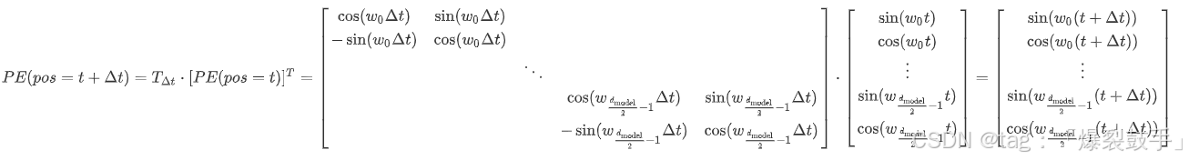
PE(pos=t) = [sin(w_0·t),cos(w_0·t)...,sin(w_{\frac{d_{model}}{2}}·t),cos(w_{\frac{d_{model}}{2}}·t)]
PE(pos=t)=[sin(w0⋅t),cos(w0⋅t)...,sin(w2dmodel⋅t),cos(w2dmodel⋅t)]
P E ( p o s = t + Δ t ) = [ s i n ( w 0 ⋅ ( t + Δ t ) ) , c o s ( w 0 ⋅ ( ( t + Δ t ) ) ) . . . , s i n ( w d m o d e l 2 ⋅ ( t + Δ t ) ) , c o s ( w d m o d e l 2 ⋅ ( t + Δ t ) ) ] \small PE(pos=t + Δt) = [sin(w_0·(t + Δt)),cos(w_0·((t + Δt)))...,sin(w_{\frac{d_{model}}{2}}·(t + Δt)),cos(w_{\frac{d_{model}}{2}}·(t + Δt))] PE(pos=t+Δt)=[sin(w0⋅(t+Δt)),cos(w0⋅((t+Δt)))...,sin(w2dmodel⋅(t+Δt)),cos(w2dmodel⋅(t+Δt))]
于是,我们可以利用旋转变换来表示 第t个Token与其他Token之间的位置关系,如下所示
位置编码的性质
- 三角编码的点积大小可以反应Token之间的距离
- 位置编码的点积是无向的
位置编码存在的问题: 进入attention层之后,内积的**距离意识(distance-aware)**的模式也遭到了破坏。
本部分参考:
Transformer学习笔记一:Positional Encoding(位置编码)
Transformer 位置编码汇总
漫谈 Transformer 中的绝对位置编码、相对位置编码和融合位置编码(旋转位置编码 RoPE)
同时,论文中也提到了作者曾经尝试使用其他形式的位置编码,比如可学习的位置编码。但后续选择使用正弦位置编码是因为它能够外拓到更长的序列长度中(对未登录的长序列样本具备更好的表现)
“We also experimented with using learned positional embeddings [8] instead, and found that the two versions produced nearly identical results (see Table 3 row (E)). We chose the sinusoidal version because it may allow the model to extrapolate to sequence lengths longer than the ones encountered during training”
Positional Embedding的实现代码实现
# todo:定义位置编码类 `PositionalEncoding`
class PositionalEncoding(nn.Module):
    __doc__ = """
        位置编码器(Positional Encoding)是Transformer模型中的一个重要组成部分,用于在模型中引入序列中各个元素的位置或顺序信息。
        因为在Transformer的编码器结构中, 并没有RNN那样针对词汇位置信息的处理能力,它无法直接感知输入数据中的顺序关系。
        因此需要在Embedding层后加入位置编码器,将词汇位置不同可能会产生不同语义的信息加入到词嵌入张量中, 以弥补位置信息的缺失。
        位置编码器将序列位置(例如,单词在句子中的位置)转换为一组向量,这些向量会与输入的词嵌入(word embeddings)相加,使模型能够在处理每个词时,理解其在序列中的位置。
        位置编码通常使用正弦和余弦函数生成,使得模型可以区分不同位置的token。
            # 手动实现`transformer`中的位置编码层
                ## 实现思路
                    1.生成一个全0张量矩阵 PE(max_len, d_model)
                    2.计算位置编码矩阵
                        torch.sin(position / (10000 ** (_2i / self.d_model)))
                        torch.cos(position / (10000 ** (_2i / self.d_model)))
                    3. 将位置编码信息与传入的样本相加并返回
                        x = x + self.PE[:, :x.shape[1], :]
            """

    def __init__(self, d_model, dropout_p, max_len=5000):
        """
        :param d_model:词向量维度
        :param dropout_p:dropout正则化概率
        :param max_len:句子的最大长度
        """
        super(PositionalEncoding, self).__init__()
        # todo:0- 初始化参数
        self.d_model = d_model
        self.max_len = max_len
        self.dropout_p = dropout_p

        # todo:1- 定义`dropout`层
        self.dropout = nn.Dropout(p=self.dropout_p)

        """
        # 位置编码公式
            PE_{(pos,2i)} = sin(\frac{pos}{10000 ** (2i/d_model)}
            PE_{(pos,2i+1)} = cos(\frac{pos}{10000 ** (2i/d_model)}
        思路:位置编码矩阵 + 特征矩阵 相当于给特征增加了位置信息
        定义位置编码矩阵PE eg pe[60, 512], 位置编码矩阵和特征矩阵形状是一样的
        """
        # todo:2- 定义位置编码矩阵
        PE = torch.zeros(max_len, d_model)

        # todo:3- 定义位置列矩阵`position`
        # 数据形状[max_len,1] eg: [0,1,2,3,4...60]^T
        position = torch.arange(0, self.max_len).unsqueeze(1)

        # todo:4- 计算 `2i` => 词向量的位置索引
        _2i = torch.arange(0, self.d_model, step=2)
        # print('_2i->',_2i)

        # todo:5- 计算位置编码矩阵:方式一
        PE[:, 0::2] = torch.sin(position / (10000 ** (_2i / self.d_model)))
        PE[:, 1::2] = torch.cos(position / (10000 ** (_2i / self.d_model)))

        # # todo:5- 计算位置编码矩阵:方式二
        # div_term = torch.exp(-torch.arange(0, d_model, 2) / d_model * math.log(10000.0))
        # PE[:, 0::2] = torch.sin(position * div_term)
        # PE[:, 1::2] = torch.cos(position * div_term)

        # todo:6- 将二维的位置编码矩阵`PE`在0轴升维, 词向量是三维 =>(1,max_len, d_model)

        PE = PE.unsqueeze(0)
        # todo:7- 将结果保存缓存区, 后续使用直接按模型参数加载
        self.register_buffer('PE', PE)

        # print('PE->', self.PE.shape, self.PE)

    # todo: 定义`forward`前向传播函数
    def forward(self, x):
        """
        x.shape -> (batch_size,seq_len,d_model)
        :param x: x->词嵌入层后的词向量
        :return: x + self.PE[:, :x.shape[1], :] => 位置编码后的结果
        """
        # 第1个 `:` -> 句子数  eg:我爱你
        # `:x.shape[1]` -> 句子长度  :3
        # 第2个 `:` -> 位置编码信息
        x = x + self.PE[:, :x.shape[1], :]
        return self.dropout(x)