Latex是一种高质量的排版系统,尤其擅长于数学公式的排版。本文我将带大家深入了解Latex在数学公式排版中的应用。从基础的数学符号到复杂的公式布局,我们都会一一讲解,通过本文的学习,你将能够轻松编写出清晰、美观的数学公式,让你的学术成果更加专业!
Latex环境配置
Latex环境的配置主要涉及到TexLive和TexStudio的安装,还未安装额小伙伴可以看我之前发布的这篇教程文章
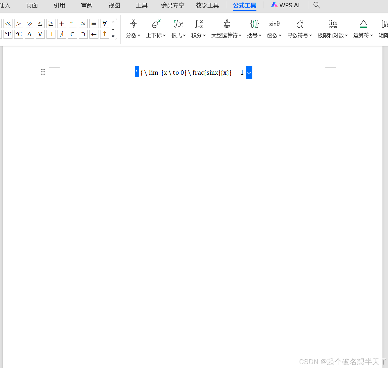
https://blog.csdn.net/weixin_73953650/article/details/147006037?spm=1001.2014.3001.5501![]() https://blog.csdn.net/weixin_73953650/article/details/147006037?spm=1001.2014.3001.5501 这里我们要说明的是就数学公式而言,不是必须使用Texstudio才可以书写,目前Word和Wps中都支持Latex语法书写公式。本文我们的Latex环境为TexStudio。
https://blog.csdn.net/weixin_73953650/article/details/147006037?spm=1001.2014.3001.5501 这里我们要说明的是就数学公式而言,不是必须使用Texstudio才可以书写,目前Word和Wps中都支持Latex语法书写公式。本文我们的Latex环境为TexStudio。

Latex环境声明
在 LaTeX 中,\begin{} 和 \end{} 是用于定义环境(environment)的关键命令,它们总是成对出现,用于控制特定范围内的文本格式、布局或行为。
| 环境名称 | 用途 | 示例 |
|---|---|---|
document | 文档主体(必须存在) | \begin{document} 文章内容 \end{document} |
itemize | 无序列表 | \begin{itemize} \item 项目1 \item 项目2 \end{itemize} |
enumerate | 有序列表 | \begin{enumerate} \item 第一项 \item 第二项 \end{enumerate} |
center | 居中对齐文本 | \begin{center} 居中内容 \end{center} |
table | 表格环境 | \begin{table}[h] \caption{标题} 表格内容 \end{table} |
figure | 图片环境 | \begin{figure}[h] \includegraphics{image.png} \end{figure} |
equation | 编号的数学公式 | \begin{equation} E=mc^2 \end{equation} |
align | 多行对齐公式(需amsmath) | \begin{align} x &= y + z \\ a &= b \end{align} |
verbatim | 原样输出(忽略LaTeX命令) | \begin{verbatim} \textbf{不会加粗} \end{verbatim} |
基本语法
\begin{环境名称}
    %环境内容
\end{环境名称}
数学公式分类
Latex中数学公式可以分为两类,分别是行内公式与行间公式。
行内公式
行内公式是指公式嵌入在文本行中,与文字在同一行显示。在Latex中使用单个$(shift+4)符号包裹。
语法
$公式$示例
\documentclass[UTF8]{ctexart}
\usepackage{fancyhdr}
\pagestyle{fancy}
\fancyhf{}
\cfoot{\thepage}
\setlength{\parskip}{0.5\baselineskip}
\begin{document}
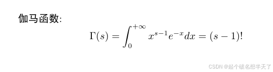
\textbf{伽马函数}:$\Gamma(s)=\int_{0}^{+\infty}x^{s-1}e^{-x}dx=(s-1)!$\\
对于$\int_{0}^{+\infty}3x^{11}e^{-x^{3}}dx$,利用凑微分的基本思想,我们不难得到\\
原式=$\int_0^+\infty(x^{3})^{3}e^{-x^{3}}dx^{3}=\Gamma(4)=3!=6$
\end{document}结果

行间公式
行间公式是指公式单独占据一行,居中显示,通常更大、更突出。在Latex中使用一对$(shift+4)符号包裹。
语法
$$公式$$示例
\documentclass[UTF8]{ctexart}
\usepackage{fancyhdr}
\pagestyle{fancy}
\fancyhf{}
\cfoot{\thepage}
\setlength{\parskip}{0.5\baselineskip}
\begin{document}
	\textbf{伽马函数}:$$\Gamma(s)=\int_{0}^{+\infty}x^{s-1}e^{-x}dx=(s-1)!$$
\end{document}
结果
数学公式语法
我们都知道数学公式无非就是数学运算符和其内部变量的组合,在Latex中也是如此,因此这里我将其分为这两个部分来进行讲解。
数学运算符
在Latex中数学运算符的一般语法格式是:
\运算符英文名称当运算符英文名称过长的时候我们一般都使用其缩写,比如分式(fraction),其Latex语法格式为:
\frac{分子}{分母}这里,我将常用的数学运算符按照其功能分为以下几类;
基本运算符
| 运算符名称 | LaTeX 表达式 | 示例(LaTeX 代码) | 显示效果 |
|---|---|---|---|
| 加号 | + | a + b | a+b |
| 减号 | - | c - d | c−d |
| 乘号(点乘) | \cdot | x \cdot y | x⋅y |
| 乘号(叉乘) | \times | a \times b | a×b |
| 除号(斜杠) | / | a / b | a/b |
| 除号(分数形式) | \frac{a}{b} | \frac{x}{y} | |
| 等于号 | = | a = b | a=b |
| 不等于 | \neq | a \neq b | a!=b |
| 约等于 | \approx | x \approx y | x≈y |
| 大于 | > | a > b | a>b |
| 小于 | < | c < d | c<d |
| 大于等于 | \geq | x \geq y | x≥y |
| 小于等于 | \leq | p \leq q | p≤q |
| 正比于 | \propto | y \propto x | y∝x |
| 求和 | \sum | \sum_{i=1}^n i | |
| 求积 | \prod | \prod_{k=1}^n k | |
| 积分 | \int | \int_a^b f(x) dx | |
| 极限 | \lim | \lim_{x \to \infty} f(x) | |
| 无穷大 | \infty | x \to \infty | x→∞ |
| 梯度(Nabla) | \nabla | \nabla f | ∇f |
| 偏导数 | \partial | \frac{\partial f}{\partial x} | |
| 根号 | \sqrt{x} | \sqrt{a^2+b^2} | |
| n次方根 | \sqrt[n]{x} | \sqrt[3]{8} | |
| 绝对值 | \vert x \vert | \vert a - b \vert | ∣a−b∣ |
| 范数 | | x | | | \mathbf{v} | | ∥v∥ |
| 因为 | \because | \because | |
| 所以 | \therefore | \therefore | |
| 函数 | \函数名(自变量) | \ln(x) |
括号运算符
| 类型 | LaTeX 表达式 | 示例效果 |
|---|---|---|
| 基本括号 | ||
| 圆括号 | (a + b) | (a+b) |
| 方括号 | [x, y] | [x,y] |
| 花括号 | \{a, b\} | {a,b} |
| 尖括号 | \langle \phi | \psi \rangle | ⟨ϕ∥ψ⟩ |
| 自适应括号 | ||
| 自动调整大小 | \left( \frac{a}{b} \right) | (ba) |
| 手动指定大小 | \big( \Big( \bigg( \Bigg( | (((( |
| 矩阵环境 | ||
基础矩阵(matrix) | \begin{matrix} a & b \\ c & d \end{matrix} | |
带括号矩阵(pmatrix) | \begin{pmatrix} a & b \\ c & d \end{pmatrix} | |
带方括号矩阵(bmatrix) | \begin{bmatrix} 1 & 0 \\ 0 & 1 \end{bmatrix} | |
带花括号矩阵(Bmatrix) | \begin{Bmatrix} x & y \\ z & w \end{Bmatrix} | |
行列式(vmatrix) | \begin{vmatrix} a & b \\ c & d \end{vmatrix} | |
范数(Vmatrix) | \begin{Vmatrix} \mathbf{u} & \mathbf{v} \end{Vmatrix} | |
矩阵运算符
| 转置 | A^\top 或 A^\intercal | A⊤, A⊺ |
| 共轭转置 | A^\dagger | A† |
| 逆矩阵 | A^{-1} | A−1 |
| 矩阵乘法 | A \times B 或 A \cdot B | A×B, A⋅B |
| 克罗内克积(Kronecker) | A \otimes B | A⊗B |
| 哈达玛积(逐元素乘) | A \circ B | A∘B |
| 直和 | A \oplus B | A⊕B |
| 迹(Trace) | \operatorname{tr}(A) | tr(A) |
| 行列式(Det) | \det(A) | det(A) |
| 范数 | | A | 或 | A |_F(Frobenius范数) | ∥A∥, ∥A∥F |
逻辑运算符
| 名称 | LaTeX 表达式 | 示例(LaTeX 代码) | 显示效果 |
|---|---|---|---|
| 逻辑与(合取) | \land | A \land B | A∧B |
| 逻辑或(析取) | \lor | A \lor B | A∨B |
| 逻辑非(否定) | \lnot 或 \neg | \lnot P | ¬P |
| 蕴含(条件) | \to 或 \rightarrow | P \to Q | P→Q |
| 双线蕴含 | \Rightarrow | A \Rightarrow B | A⇒B |
| 等价(双条件) | \leftrightarrow | P \leftrightarrow Q | P↔Q |
| 双线等价 | \Leftrightarrow | A \Leftrightarrow B | A⇔B |
| 恒真(真值) | \top | \vdash \top | ⊢⊤ |
| 恒假(矛盾) | \bot | P \land \bot | P∧⊥ |
| 全称量词 | \forall | \forall x \in S | ∀x∈S |
| 存在量词 | \exists | \exists y > 0 | ∃y>0 |
| 推导(断定) | \vdash | \Gamma \vdash \phi | Γ⊢ϕ |
| 语义蕴含 | \vDash | A \vDash B | A⊨B |
| 模型满足 | \models | \mathcal{M} \models T | M⊨T |
| 异或(不可兼或) | \oplus | A \oplus B | A⊕B |
| 同或(XNOR) | \odot | A \odot B | A⊙B |
| 集合差 | \setminus | A \setminus B | A∖B |


![[Python] 企业内部应用接入钉钉登录,端内免登录+浏览器授权登录](https://i-blog.csdnimg.cn/direct/640ce48397194d80bae2f77f830f5b55.png)