1. 快速入门python,python基本语法
Python使用缩进(tab或者空格)来组织代码,而不是像其 他语言比如R、C++、Java和Perl那样用大括号。考虑使用for循 环来实现排序算法:
   for x in list_values:
       if x < 10:
           small.append(x)
       else:
           bigger.append(x)
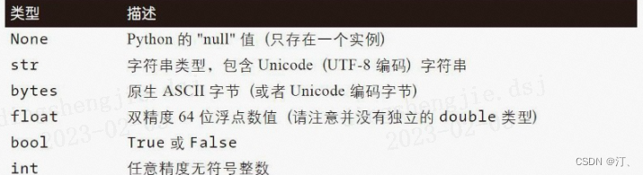
标量类型
2.3,4,null,True都是标量
变量
a=2
b='this is alibaba'
c=[1,2,456.,np.nan,c]
数据结构
#列表(list)
myList=[1,2,"hello bro",np.nan,3456225.0987]
#元组(tuple,不可修改)
myTuple=(2,3,'hey morning!',89,np.nan)
#字典(dictionary,俗称键值对)
myDictionary={'key1' :23, "key2" : "hahahh,哈哈哈", "key3" : 78}
#集合(set,集合)
myset=set({'happy','sad','sad'})
运算
a=8
b=2
c=a**b
d=a/b
d
函数(打包好的功能块)
#定义一个计算平均数的函数
def get_avg(values):
    if len(values) == 0:#如果输入的list没有值
        return 0 #返回0

    sum_v = 0
    #遍历所有值
    for value in values:
        #前一个和加上后一个值
        sum_v = value+sum_v
    return sum_v / len(values)

avg = get_avg([1, 2, 3, 4])
avg
def get_avg(values):
    if len(values) == 0:#如果输入的list没有值
        return 0 #返回0

    sum_v = 0
    #遍历所有值
    for value in values:
        #前一个和加上后一个值
        sum_v = value+sum_v
    return sum_v / len(values)

avg = get_avg([1, 2, 3, 4])
avg
循环
sum10 = 0
for i in range(1, 11):
    sum10 = sum10+i
print(sum10)
sum10 = 0
for i in range(1, 11):
    sum10 = sum10+i
    print(i)
print(sum10)
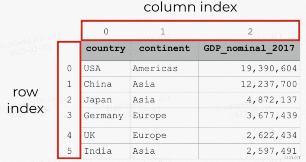
2. 快速入门pandas
2.1 pandas核心数据结构和常用API
pandas资料下载链接:https://download.csdn.net/download/sinat_39620217/87413329


2.2 pandas 基础数据操作
导入常用的数据分析库
import numpy as np
import pandas as pd
#创建一个series
s = pd.Series([1, 3, 5, np.nan, 6, 8])
s

0    1.0
1    3.0
2    5.0
3    NaN
4    6.0
5    8.0
dtype: float64
#创建一个时间序列
dates = pd.date_range("20130101", periods=6)
dates

DatetimeIndex(['2023-02-03', '2023-02-04', '2023-02-05', '2023-02-06',
               '2023-02-07', '2023-02-08'],
              dtype='datetime64[ns]', freq='D')
#以时间序列为index,以“ABCD”为列明,用24个符合正态分布的随机数作为数值
df = pd.DataFrame(np.random.randn(6, 4), index=dates, columns=list("ABCD"))
df

	A	B	C	D
2023-02-03	-1.688539	-0.687145	-0.087825	-0.113740
2023-02-04	-0.483402	-2.333871	-1.078778	1.786806
2023-02-05	1.154374	0.976104	0.004643	0.754242
2023-02-06	-0.005039	-0.170111	0.578378	0.604114
2023-02-07	1.923344	-1.132254	1.408248	0.101545
2023-02-08	0.876144	1.589423	1.678817	-1.271310
#另一种创建df的方法
df2 = pd.DataFrame(
    {
        "A": 1.0,
        "B": pd.Timestamp("20130102"),
        "C": pd.Series(1, index=list(range(4)), dtype="float32"),
        "D": np.array([3] * 4, dtype="int32"),
        "E": pd.Categorical(["test", "train", "test", "train"]),
        "F": "foo",
    }
)
df2

     A          B    C  D      E    F
0  1.0 2013-01-02  1.0  3   test  foo
1  1.0 2013-01-02  1.0  3  train  foo
2  1.0 2013-01-02  1.0  3   test  foo
3  1.0 2013-01-02  1.0  3  train  foo
#看下数据类型
df2.dtypes

A           float64
B    datetime64[ns]
C           float32
D             int32
E          category
F            object
dtype: object

df2.head(2)

df2.tail()

df2.sample(3)

     A          B    C  D      E    F
0  1.0 2013-01-02  1.0  3   test  foo
1  1.0 2013-01-02  1.0  3  train  foo

     A          B    C  D      E    F
0  1.0 2013-01-02  1.0  3   test  foo
1  1.0 2013-01-02  1.0  3  train  foo
2  1.0 2013-01-02  1.0  3   test  foo
3  1.0 2013-01-02  1.0  3  train  foo

     A          B    C  D      E    F
1  1.0 2013-01-02  1.0  3  train  foo
2  1.0 2013-01-02  1.0  3   test  foo
0  1.0 2013-01-02  1.0  3   test  foo
#导入本地数据到python内存
diamonds_df=pd.read_csv('data/diamonds.csv')
diamonds_df

	carat	cut	color	clarity	depth	table	price	x	y	z
0	0.23	Ideal	E	SI2	61.5	55.0	326	3.95	3.98	2.43
1	0.21	Premium	E	SI1	59.8	61.0	326	3.89	3.84	2.31
2	0.23	Good	E	VS1	56.9	65.0	327	4.05	4.07	2.31
3	0.29	Premium	I	VS2	62.4	58.0	334	4.20	4.23	2.63
4	0.31	Good	J	SI2	63.3	58.0	335	4.34	4.35	2.75
...	...	...	...	...	...	...	...	...	...	...
53935	0.72	Ideal	D	SI1	60.8	57.0	2757	5.75	5.76	3.50
53936	0.72	Good	D	SI1	63.1	55.0	2757	5.69	5.75	3.61
53937	0.70	Very Good	D	SI1	62.8	60.0	2757	5.66	5.68	3.56
53938	0.86	Premium	H	SI2	61.0	58.0	2757	6.15	6.12	3.74
53939	0.75	Ideal	D	SI2	62.2	55.0	2757	5.83	5.87	3.64
53940 rows × 10 columns
#查看数据的信息或者基本情况
diamonds_df.info()
<class 'pandas.core.frame.DataFrame'>
RangeIndex: 53940 entries, 0 to 53939
Data columns (total 10 columns):
 #   Column   Non-Null Count  Dtype
---  ------   --------------  -----
 0   carat    53940 non-null  float64
 1   cut      53940 non-null  object
 2   color    53940 non-null  object
 3   clarity  53940 non-null  object
 4   depth    53940 non-null  float64
 5   table    53940 non-null  float64
 6   price    53940 non-null  int64
 7   x        53940 non-null  float64
 8   y        53940 non-null  float64
 9   z        53940 non-null  float64
dtypes: float64(6), int64(1), object(3)
memory usage: 4.1+ MB

#查看索引
diamonds_df.index

RangeIndex(start=0, stop=53940, step=1)


#查看列名
diamonds_df.columns

Index(['carat', 'cut', 'color', 'clarity', 'depth', 'table', 'price', 'x', 'y',
       'z'],
      dtype='object')
#查看数据基本情况
diamonds_df.describe()

	carat	depth	table	price	x	y	z
count	53940.000000	53940.000000	53940.000000	53940.000000	53940.000000	53940.000000	53940.000000
mean	0.797940	61.749405	57.457184	3932.799722	5.731157	5.734526	3.538734
std	0.474011	1.432621	2.234491	3989.439738	1.121761	1.142135	0.705699
min	0.200000	43.000000	43.000000	326.000000	0.000000	0.000000	0.000000
25%	0.400000	61.000000	56.000000	950.000000	4.710000	4.720000	2.910000
50%	0.700000	61.800000	57.000000	2401.000000	5.700000	5.710000	3.530000
75%	1.040000	62.500000	59.000000	5324.250000	6.540000	6.540000	4.040000
max	5.010000	79.000000	95.000000	18823.000000	10.740000	58.900000	31.800000

#行列转换
df.T

	2023-02-03	2023-02-04	2023-02-05	2023-02-06	2023-02-07	2023-02-08
A	-1.688539	-0.483402	1.154374	-0.005039	1.923344	0.876144
B	-0.687145	-2.333871	0.976104	-0.170111	-1.132254	1.589423
C	-0.087825	-1.078778	0.004643	0.578378	1.408248	1.678817
D	-0.113740	1.786806	0.754242	0.604114	0.101545	-1.271310
2.3 pandas多维度排序
#对数据进行排序
df.sort_values(by="B",ascending=False)
diamonds_df.head()

	A	B	C	D
2023-02-08	0.876144	1.589423	1.678817	-1.271310
2023-02-05	1.154374	0.976104	0.004643	0.754242
2023-02-06	-0.005039	-0.170111	0.578378	0.604114
2023-02-03	-1.688539	-0.687145	-0.087825	-0.113740
2023-02-07	1.923344	-1.132254	1.408248	0.101545
2023-02-04	-0.483402	-2.333871	-1.078778	1.786806
 #按照cut和color联合排序
diamonds_df.sort_values(by=['cut','color','price'],ascending=False)

	carat	cut	color	clarity	depth	table	price	x	y	z
27586	2.44	Very Good	J	VS2	58.1	60.0	18430	8.89	8.93	5.18
27352	2.39	Very Good	J	VS1	59.6	60.0	17920	8.71	8.77	5.21
27185	2.44	Very Good	J	SI1	62.9	53.0	17472	8.58	8.62	5.41
27024	2.74	Very Good	J	SI2	61.5	62.0	17164	8.87	8.90	5.46
26958	2.50	Very Good	J	SI1	62.8	57.0	17028	8.58	8.65	5.41
...	...	...	...	...	...	...	...	...	...	...
28534	0.42	Fair	D	SI1	64.7	61.0	675	4.70	4.73	3.05
25695	0.40	Fair	D	SI1	65.1	55.0	644	4.63	4.68	3.03
10380	0.29	Fair	D	VS2	64.7	62.0	592	4.14	4.11	2.67
2711	0.25	Fair	D	VS1	61.2	55.0	563	4.09	4.11	2.51
48630	0.30	Fair	D	SI2	64.6	54.0	536	4.29	4.25	2.76
53940 rows × 10 columns
2.4 pandas数据筛选
#列范围
diamonds_df[["cut","depth","price"]]

	cut	depth	price
0	Ideal	61.5	326
1	Premium	59.8	326
2	Good	56.9	327
3	Premium	62.4	334
4	Good	63.3	335
#行范围
diamonds_df[6:9]

	carat	cut	color	clarity	depth	table	price	x	y	z
6	0.24	Very Good	I	VVS1	62.3	57.0	336	3.95	3.98	2.47
7	0.26	Very Good	H	SI1	61.9	55.0	337	4.07	4.11	2.53
8	0.22	Fair	E	VS2	65.1	61.0	337	3.87	3.78	2.49
#按行范围和列具体
diamonds_df.loc[5:9, ["carat","price","x"]]

	carat	price	x
5	0.24	336	3.94
6	0.24	336	3.95
7	0.26	337	4.07
8	0.22	337	3.87
9	0.23	338	4.00
#按行具体和列范围
#注意:具体必须要用list来承载(中括号),范围不能用中括号
diamonds_df.loc[[3,6,9], "cut":"price"]


cut	color	clarity	depth	table	price
3	Premium	I	VS2	62.4	58.0	334
6	Very Good	I	VVS1	62.3	57.0	336
9	Very Good	H	VS1	59.4	61.0	338
#按行逻辑和列范围
diamonds_df.loc[diamonds_df.carat>0.3, ["carat","price"]]

	carat	price
4	0.31	335
13	0.31	344
15	0.32	345
23	0.31	353
24	0.31	353
...	...	...
#按条件筛选
#按照某列进行筛选
diamonds_df[(diamonds_df["carat"] > 0.3) & (diamonds_df["price"] < 400)]

	carat	cut	color	clarity	depth	table	price	x	y	z
4	0.31	Good	J	SI2	63.3	58.0	335	4.34	4.35	2.75
13	0.31	Ideal	J	SI2	62.2	54.0	344	4.35	4.37	2.71
15	0.32	Premium	E	I1	60.9	58.0	345	4.38	4.42	2.68
23	0.31	Very Good	J	SI1	59.4	62.0	353	4.39	4.43	2.62
24	0.31	Very Good	J	SI1	58.1	62.0	353	4.44	4.47	2.59
28271	0.32	Good	D	I1	64.0	54.0	361	4.33	4.36	2.78
28277	0.31	Very Good	J	SI1	61.9	59.0	363	4.28	4.32	2.66
28278	0.31	Very Good	J	SI1	62.7	59.0	363	4.29	4.32	2.70
28279	0.31	Premium	J	SI1	60.9	60.0	363	4.36	4.38	2.66
28280	0.31	Good	J	SI1	63.5	55.0	363	4.30	4.33	2.74
#筛选cut属于Premium和Good
diamonds_df[(diamonds_df['cut'].isin(['Premium','Good'])) &
            (diamonds_df['carat']>0.3) & (diamonds_df['price']<400) ]

	carat	cut	color	clarity	depth	table	price	x	y	z
4	0.31	Good	J	SI2	63.3	58.0	335	4.34	4.35	2.75
15	0.32	Premium	E	I1	60.9	58.0	345	4.38	4.42	2.68
28271	0.32	Good	D	I1	64.0	54.0	361	4.33	4.36	2.78
28279	0.31	Premium	J	SI1	60.9	60.0	363	4.36	4.38	2.66
28280	0.31	Good	J	SI1	63.5	55.0	363	4.30	4.33	2.74
28284	0.32	Premium	J	SI1	62.2	59.0	365	4.37	4.41	2.73
34928	0.32	Good	J	SI1	63.2	56.0	374	4.31	4.36	2.74
34929	0.32	Good	I	SI2	63.4	56.0	374	4.34	4.37	2.76
34932	0.32	Good	I	SI2	63.1	58.0	374	4.34	4.41	2.76
34939	0.31	Good	I	SI1	64.3	55.0	377	4.27	4.29	2.75
2.5 pandas分组计算
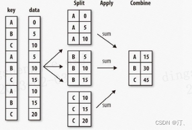
#分组计算
df = pd.DataFrame(
    {
        "A": ["foo", "bar", "foo", "bar", "foo", "bar", "foo", "foo"],
        "B": ["one", "one", "two", "three", "two", "two", "one", "three"],
        "C": np.random.randn(8),
        "D": np.random.randn(8),
    }
)
df

	A	B	C	D
0	foo	one	-1.265302	-1.718949
1	bar	one	-0.814010	0.097433
2	foo	two	-1.359590	0.708358
3	bar	three	0.562501	-2.525745
4	foo	two	1.036076	0.455022
5	bar	two	2.192717	-0.163239
6	foo	one	0.623262	-0.632277
7	foo	three	-0.791469	1.801869
#按照A分组,分别计算C和D的和
df.groupby("A")[["C", "D"]].sum()

	C	D
A
bar	1.941208	-2.591551
foo	-1.757023	0.614024
#按照多列进行分组计算
df.groupby(["A", "B"]).sum()

		C	D
A	B
bar	one	-0.814010	0.097433
three	0.562501	-2.525745
two	2.192717	-0.163239
foo	one	-0.642040	-2.351226
three	-0.791469	1.801869
two	-0.323514	1.163381
#按照cut和color的组合计算平均价格
diamonds_df.groupby(by=['cut','color'])[['price']].mean().round(2).reset_index()

	cut	color	price
0	Fair	D	4291.06
1	Fair	E	3682.31
2	Fair	F	3827.00
3	Fair	G	4239.25
4	Fair	H	5135.68
5	Fair	I	4685.45
6	Fair	J	4975.66
7	Good	D	3405.38
8	Good	E	3423.64
9	Good	F	3495.75
10	Good	G	4123.48
11	Good	H	4276.25
12	Good	I	5078.53
13	Good	J	4574.17
2.6 pandas透视表
#透视表
df = pd.DataFrame(
    {
        "甲": ["one", "one", "two", "three"] * 3,
        "乙": ["A", "B", "C"] * 4,
        "丙": ["foo", "foo", "foo", "bar", "bar", "bar"] * 2,
        "D": np.random.randn(12),
        "E": np.random.randn(12),
    }
)
df

	甲	乙	丙	D	E
0	one	A	foo	0.593815	0.399765
1	one	B	foo	0.943989	-0.073500
2	two	C	foo	0.504724	0.916902
3	three	A	bar	1.377307	0.930002
4	one	B	bar	0.364403	2.430547
5	one	C	bar	-0.392653	-0.307336
6	two	A	foo	-0.698488	2.202757
7	three	B	foo	-2.046343	0.562993
8	one	C	foo	-0.570906	0.719652
9	one	A	bar	-1.493323	0.612229
10	two	B	bar	1.744241	0.616304
11	three	C	bar	2.337644	1.568032
pd.pivot_table(df, values="D", index=["甲","乙"], columns=["丙"],aggfunc='mean')

	丙	bar	foo
甲	乙
one	A	-1.493323	0.593815
B	0.364403	0.943989
C	-0.392653	-0.570906
three	A	1.377307	NaN
B	NaN	-2.046343
C	2.337644	NaN
two	A	NaN	-0.698488
B	1.744241	NaN
C	NaN	0.504724