导向滤波
一、介绍
-
导向滤波又称引导滤波,通过一张引导图片反映边缘、物体等信息,对输入图像进行滤波处理,使输出图像的内容由输入图像决定,但纹理与引导图片相似。
-
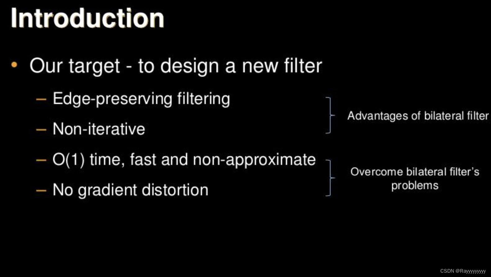
导向滤波的原理是局部线性模型,在保持双边滤波的优势(有效保持边缘,非迭代计算)的同时计算速度很快,从而克服双边滤波速度慢的缺点。
-
导向滤波(引导滤波)不仅能实现双边滤波的边缘平滑,而且在检测到边缘附近有很好的表现,可应用在图像增强、HDR压缩、图像抠图及图像去雾等场景。
-
在进行保持边缘滤波时,可以采用原始图像自身或其预处理后的图像作为导向图片。
二、对比双边滤波的优势
- 1.导向滤波比起双边滤波来说在边界附近效果较好;另外,它还具有 O(N) 的线性时间的速度优势。双边滤波器有非常大的计算复杂度O(N^2),但导向滤波器因为并未用到过于复杂的数学计算,有线性的计算复杂度。
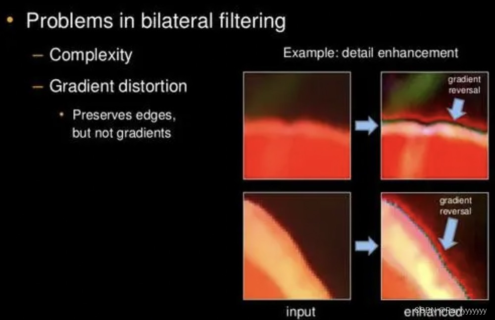
- 2.除了速度优势以外,导向滤波的一个很好的性能就是可以保持梯度,这是bilateral做不到的,因为会有梯度翻转现象。导向滤波器因为在数学上以线性组合为基础出发,输出图片(Output Image)与引导图片(Guidance Image)的梯度方向一致,不会出现梯度反转的问题。
三、导向滤波的数学原理(比较复杂,这部分可以不看了)
这部分参考大佬的一篇文章:引导滤波/导向滤波(Guided Filter)
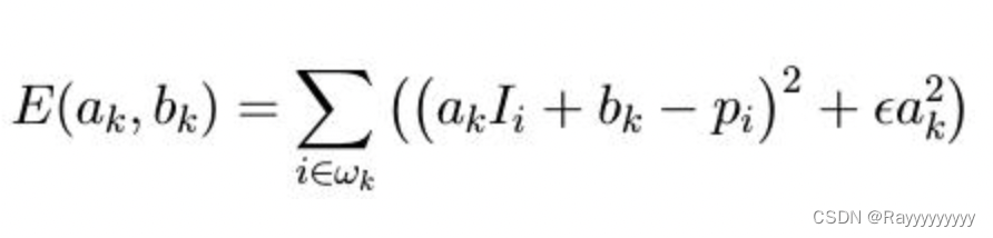
- 引导滤波的思想用一张引导图像产生权重,从而对输入图像进行处理,这个过程可以表示为下面公式:
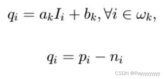
- 其中,p为输入图像,I 为导向图,q 为输出图像。在这里我们认为输出图像可以看成导向图 I 的一个局部线性变换,其中k是局部化的窗口的中点,因此属于窗口 ωk 的像素,都可以用导向图对应的像素通过(ak,bk)的系数进行变换计算出来。同时,我们认为输入图像 p 是由 q 加上我们不希望的噪声或纹理得到的,因此有 p = q + n 。
接下来就是解出这样的系数,使得p和q的差别尽量小,而且还可以保持局部线性模型。这里利用了带有正则项的 linear ridge regression(岭回归)
- 求解以上方程得到a和b在局部的值,对于一个要求的像素可能含在多个窗口中,因此平均后得到:
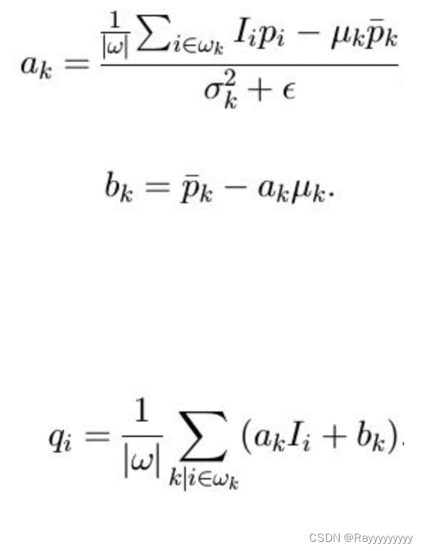
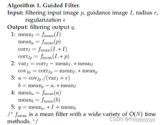
- 最终得到算法:
四、OpenGL实现导向滤波
-
这里把原图当做导向图。那么上图算法中的I=P,于是方差和协方差是相等的。
-
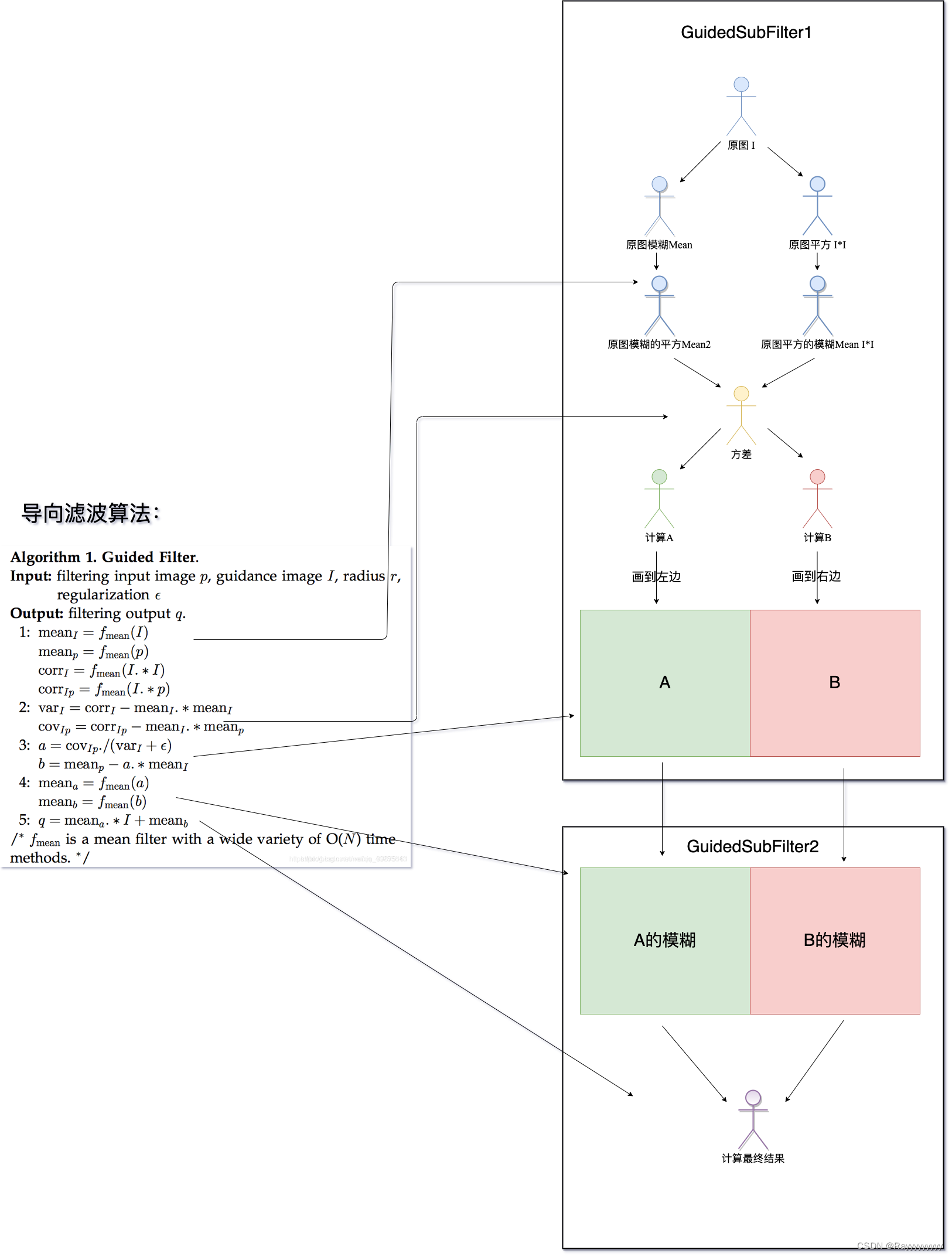
按照上面的算法,由于导向滤波需要把原始图片分别绘制a和b,还需要计算a和b的模糊图。为了节省绘制次数,把整个大算法分成2次渲染,第一次渲染求得a和b,第二次渲染求得最终的结果q
-
思路如下图:
-
为了在2次draw call内完成导向滤波操作,这里用了一个比较巧妙的方式是,在通一个绘制里同时绘制a和b的结果,把它分别画到画布的左半边和右半边(当然也可以分成上下)。
- 需要注意的是这个画布的宽需要原始图片宽的2倍大,在创建纹理的时候需要注意纹理的尺寸
-
以下为2次绘制的opengl shader
-
GuidedSubFilter1 片源着色器:
precision highp float;

uniform sampler2D u_origin; // 原图
varying vec2 texcoordOut;

uniform vec2 offset;  // 单个像素步长
uniform float alpha;   // 模糊程度
uniform float eps;   // 正则化参数e

// 均值模糊,5*5
vec3 meanBlur(vec3 colors[25]) {
    highp vec3 sum = vec3(0.0);
    for (int i = 0; i < 25; i++) {
        sum += colors[i];
    }
    return sum * 0.04;
}

void main()
{
    // 因为这个shader最终画到一个 2*w, h 尺寸的一个FBO上,左边是导向滤波的a结果,右边是导向滤波的b结果,所以这里需要计算在原始纹理上真实的采样坐标
    highp vec2 originTexcoord;
    if (texcoordOut.x < 0.5) {
        originTexcoord = vec2(texcoordOut.x * 2.0, texcoordOut.y);
    } else {
        originTexcoord = vec2((texcoordOut.x - 0.5) * 2.0, texcoordOut.y);
    }

    // 采样原图 I 的 5*5 个点
    highp vec3 origin[25];

    origin[0] = texture2D(u_origin, originTexcoord).rgb;

    origin[1] = texture2D(u_origin, originTexcoord + vec2(offset.x, 0.0)).rgb;
    origin[2] = texture2D(u_origin, originTexcoord + vec2(-offset.x, 0.0)).rgb;
    origin[3] = texture2D(u_origin, originTexcoord + vec2(0.0, offset.y)).rgb;
    origin[4] = texture2D(u_origin, originTexcoord + vec2(0.0, -offset.y)).rgb;

    origin[5] = texture2D(u_origin, originTexcoord + vec2(offset.x, offset.y)).rgb;
    origin[6] = texture2D(u_origin, originTexcoord + vec2(offset.x, -offset.y)).rgb;
    origin[7] = texture2D(u_origin, originTexcoord + vec2(-offset.x, offset.y)).rgb;
    origin[8] = texture2D(u_origin, originTexcoord + vec2(-offset.x, -offset.y)).rgb;

    origin[9] = texture2D(u_origin, originTexcoord + vec2(2.0 * offset.x, 0)).rgb;
    origin[10] = texture2D(u_origin, originTexcoord + vec2(-2.0 * offset.x, 0)).rgb;
    origin[11] = texture2D(u_origin, originTexcoord + vec2(0, 2.0 * offset.y)).rgb;
    origin[12] = texture2D(u_origin, originTexcoord + vec2(0, -2.0 * offset.y)).rgb;

    origin[13] = texture2D(u_origin, originTexcoord + vec2(2.0 * offset.x, 2.0 * offset.y)).rgb;
    origin[14] = texture2D(u_origin, originTexcoord + vec2(2.0 * offset.x, -2.0 * offset.y)).rgb;
    origin[15] = texture2D(u_origin, originTexcoord + vec2(-2.0 * offset.x, 2.0 * offset.y)).rgb;
    origin[16] = texture2D(u_origin, originTexcoord + vec2(-2.0 * offset.x, -2.0 * offset.y)).rgb;

    origin[17] = texture2D(u_origin, originTexcoord + vec2(2.0 * offset.x, offset.y)).rgb;
    origin[18] = texture2D(u_origin, originTexcoord + vec2(-2.0 * offset.x, offset.y)).rgb;
    origin[19] = texture2D(u_origin, originTexcoord + vec2(offset.x, 2.0 * offset.y)).rgb;
    origin[20] = texture2D(u_origin, originTexcoord + vec2(-offset.x, 2.0 * offset.y)).rgb;

    origin[21] = texture2D(u_origin, originTexcoord + vec2(2.0 * offset.x, -offset.y)).rgb;
    origin[22] = texture2D(u_origin, originTexcoord + vec2(-2.0 * offset.x, -offset.y)).rgb;
    origin[23] = texture2D(u_origin, originTexcoord + vec2(offset.x, -2.0 * offset.y)).rgb;
    origin[24] = texture2D(u_origin, originTexcoord + vec2(-offset.x, -2.0 * offset.y)).rgb;

    // 计算原图的平方 I*I
    highp vec3 origin2[25];
    for (int i = 0; i < 25; i++) {
        origin2[i] = origin[i] * origin[i];
    }

    // 原图 I 的均值模糊
    highp vec3 originMean = meanBlur(origin);
    // 原图平方 I*I 的均值模糊
    highp vec3 origin2Mean = meanBlur(origin2);

    originMean = mix(origin[0], originMean, alpha);
    origin2Mean = mix(origin2[0], origin2Mean, alpha);

    // 原图模糊的平方
    highp vec3 originMean2 = originMean * originMean;

    // 计算方差(对于磨皮来说引导图和原图是同一个图,方差和协方差是同一个)
    highp vec3 variance = origin2Mean - originMean2;

    // 计算导向滤波的AB结果
    highp vec3 A = variance / (variance + eps);
    highp vec3 B = originMean - A * originMean;

    // 把AB分别写到图像的左半部分和右半部分
    if (texcoordOut.x < 0.5) {
        gl_FragColor = vec4((A + 1.0) * 0.5, 1.0);
    } else {
        gl_FragColor = vec4((B + 1.0) * 0.5, 1.0);
    }

}
- GuidedSubFilter2 片源着色器:
precision highp float;

uniform sampler2D u_origin; // 原图
uniform sampler2D u_AB;    // guided1的结果,左边是导向滤波的a结果,右边是导向滤波的b结果
varying vec2 texcoordOut;

uniform vec2 offset;  // 单个像素步长
uniform float alpha;   // 模糊程度

// 均值模糊,5*5
vec3 meanBlur(vec3 colors[25]) {
    highp vec3 sum = vec3(0.0);
    for (int i = 0; i < 25; i++) {
        sum += colors[i];
    }
    return sum * 0.04;
}

void main()
{
    // 采样图 A 的 5*5 个点
    highp vec3 colorA[25];
    highp vec2 texcoordA = vec2(texcoordOut.x * 0.5, texcoordOut.y);

    colorA[0] = texture2D(u_AB, texcoordA).rgb;

    colorA[1] = texture2D(u_AB, texcoordA + vec2(offset.x, 0.0)).rgb;
    colorA[2] = texture2D(u_AB, texcoordA + vec2(-offset.x, 0.0)).rgb;
    colorA[3] = texture2D(u_AB, texcoordA + vec2(0.0, offset.y)).rgb;
    colorA[4] = texture2D(u_AB, texcoordA + vec2(0.0, -offset.y)).rgb;

    colorA[5] = texture2D(u_AB, texcoordA + vec2(offset.x, offset.y)).rgb;
    colorA[6] = texture2D(u_AB, texcoordA + vec2(offset.x, -offset.y)).rgb;
    colorA[7] = texture2D(u_AB, texcoordA + vec2(-offset.x, offset.y)).rgb;
    colorA[8] = texture2D(u_AB, texcoordA + vec2(-offset.x, -offset.y)).rgb;

    colorA[9] = texture2D(u_AB, texcoordA + vec2(2.0 * offset.x, 0)).rgb;
    colorA[10] = texture2D(u_AB, texcoordA + vec2(-2.0 * offset.x, 0)).rgb;
    colorA[11] = texture2D(u_AB, texcoordA + vec2(0, 2.0 * offset.y)).rgb;
    colorA[12] = texture2D(u_AB, texcoordA + vec2(0, -2.0 * offset.y)).rgb;

    colorA[13] = texture2D(u_AB, texcoordA + vec2(2.0 * offset.x, 2.0 * offset.y)).rgb;
    colorA[14] = texture2D(u_AB, texcoordA + vec2(2.0 * offset.x, -2.0 * offset.y)).rgb;
    colorA[15] = texture2D(u_AB, texcoordA + vec2(-2.0 * offset.x, 2.0 * offset.y)).rgb;
    colorA[16] = texture2D(u_AB, texcoordA + vec2(-2.0 * offset.x, -2.0 * offset.y)).rgb;

    colorA[17] = texture2D(u_AB, texcoordA + vec2(2.0 * offset.x, offset.y)).rgb;
    colorA[18] = texture2D(u_AB, texcoordA + vec2(-2.0 * offset.x, offset.y)).rgb;
    colorA[19] = texture2D(u_AB, texcoordA + vec2(offset.x, 2.0 * offset.y)).rgb;
    colorA[20] = texture2D(u_AB, texcoordA + vec2(-offset.x, 2.0 * offset.y)).rgb;

    colorA[21] = texture2D(u_AB, texcoordA + vec2(2.0 * offset.x, -offset.y)).rgb;
    colorA[22] = texture2D(u_AB, texcoordA + vec2(-2.0 * offset.x, -offset.y)).rgb;
    colorA[23] = texture2D(u_AB, texcoordA + vec2(offset.x, -2.0 * offset.y)).rgb;
    colorA[24] = texture2D(u_AB, texcoordA + vec2(-offset.x, -2.0 * offset.y)).rgb;

    // 采样图 B 的 5*5 个点
    highp vec3 colorB[25];
    highp vec2 texcoordB = vec2(texcoordOut.x * 0.5 + 0.5, texcoordOut.y);

    colorB[0] = texture2D(u_AB, texcoordB).rgb;

    colorB[1] = texture2D(u_AB, texcoordB + vec2(offset.x, 0.0)).rgb;
    colorB[2] = texture2D(u_AB, texcoordB + vec2(-offset.x, 0.0)).rgb;
    colorB[3] = texture2D(u_AB, texcoordB + vec2(0.0, offset.y)).rgb;
    colorB[4] = texture2D(u_AB, texcoordB + vec2(0.0, -offset.y)).rgb;

    colorB[5] = texture2D(u_AB, texcoordB + vec2(offset.x, offset.y)).rgb;
    colorB[6] = texture2D(u_AB, texcoordB + vec2(offset.x, -offset.y)).rgb;
    colorB[7] = texture2D(u_AB, texcoordB + vec2(-offset.x, offset.y)).rgb;
    colorB[8] = texture2D(u_AB, texcoordB + vec2(-offset.x, -offset.y)).rgb;

    colorB[9] = texture2D(u_AB, texcoordB + vec2(2.0 * offset.x, 0)).rgb;
    colorB[10] = texture2D(u_AB, texcoordB + vec2(-2.0 * offset.x, 0)).rgb;
    colorB[11] = texture2D(u_AB, texcoordB + vec2(0, 2.0 * offset.y)).rgb;
    colorB[12] = texture2D(u_AB, texcoordB + vec2(0, -2.0 * offset.y)).rgb;

    colorB[13] = texture2D(u_AB, texcoordB + vec2(2.0 * offset.x, 2.0 * offset.y)).rgb;
    colorB[14] = texture2D(u_AB, texcoordB + vec2(2.0 * offset.x, -2.0 * offset.y)).rgb;
    colorB[15] = texture2D(u_AB, texcoordB + vec2(-2.0 * offset.x, 2.0 * offset.y)).rgb;
    colorB[16] = texture2D(u_AB, texcoordB + vec2(-2.0 * offset.x, -2.0 * offset.y)).rgb;

    colorB[17] = texture2D(u_AB, texcoordB + vec2(2.0 * offset.x, offset.y)).rgb;
    colorB[18] = texture2D(u_AB, texcoordB + vec2(-2.0 * offset.x, offset.y)).rgb;
    colorB[19] = texture2D(u_AB, texcoordB + vec2(offset.x, 2.0 * offset.y)).rgb;
    colorB[20] = texture2D(u_AB, texcoordB + vec2(-offset.x, 2.0 * offset.y)).rgb;

    colorB[21] = texture2D(u_AB, texcoordB + vec2(2.0 * offset.x, -offset.y)).rgb;
    colorB[22] = texture2D(u_AB, texcoordB + vec2(-2.0 * offset.x, -offset.y)).rgb;
    colorB[23] = texture2D(u_AB, texcoordB + vec2(offset.x, -2.0 * offset.y)).rgb;
    colorB[24] = texture2D(u_AB, texcoordB + vec2(-offset.x, -2.0 * offset.y)).rgb;

    // 分别对图A和图B做均值模糊
    highp vec3 meanA = meanBlur(colorA);
    highp vec3 meanB = meanBlur(colorB);

    meanA = meanA * 2.0 - 1.0;
    meanB = meanB * 2.0 - 1.0;

    meanA = mix(colorA[0] * 2.0 - 1.0, meanA, alpha);
    meanB = mix(colorB[0] * 2.0 - 1.0, meanB, alpha);

    // 导向滤波的最后一步融合
    highp vec3 originColor = texture2D(u_origin, texcoordOut).rgb;
    highp vec3 resultColor = meanA * originColor + meanB;
    resultColor = mix(originColor, resultColor, alpha);

    gl_FragColor = vec4(resultColor, 1.0);
}
绘制结果:
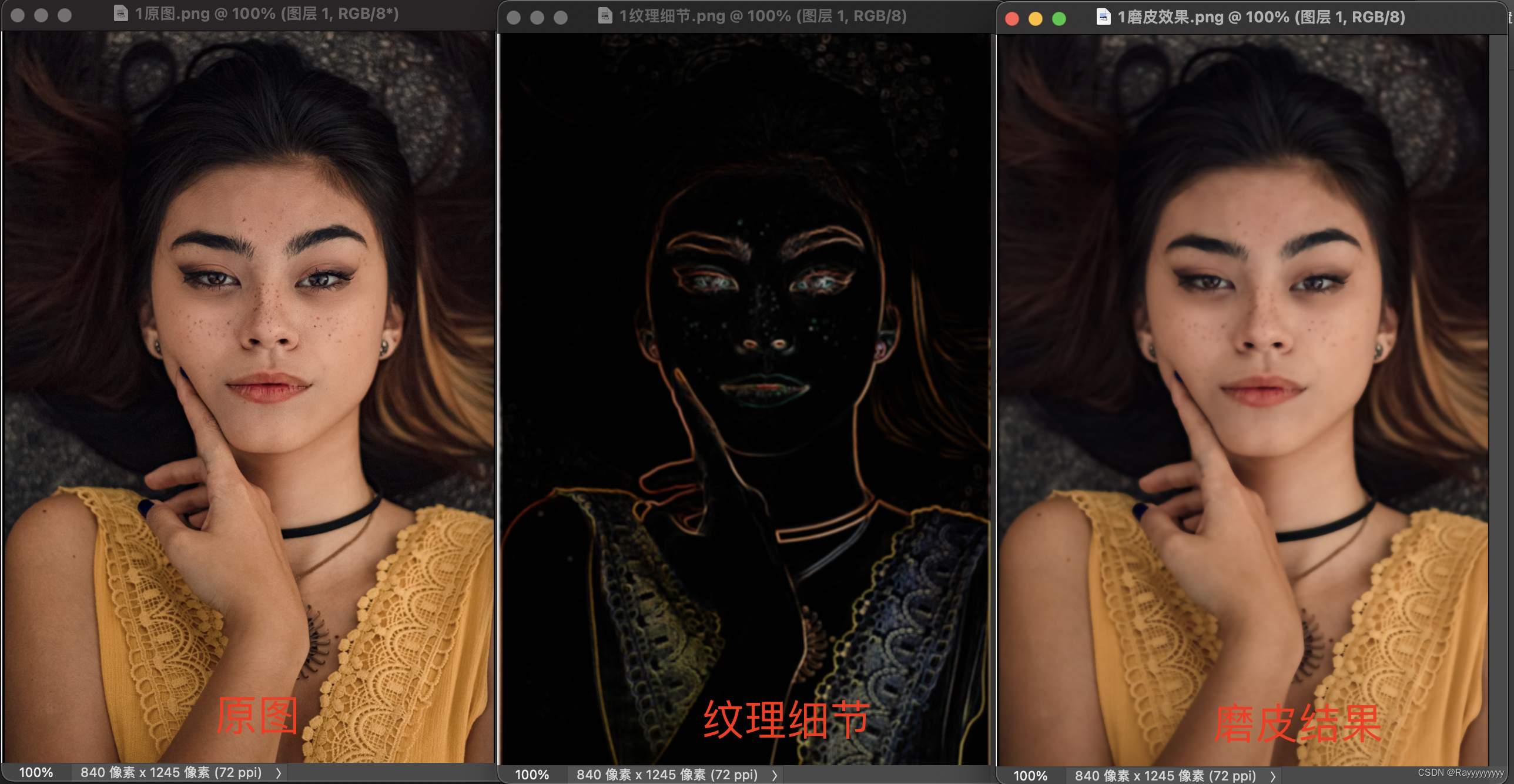 正则化参数eps=0.02
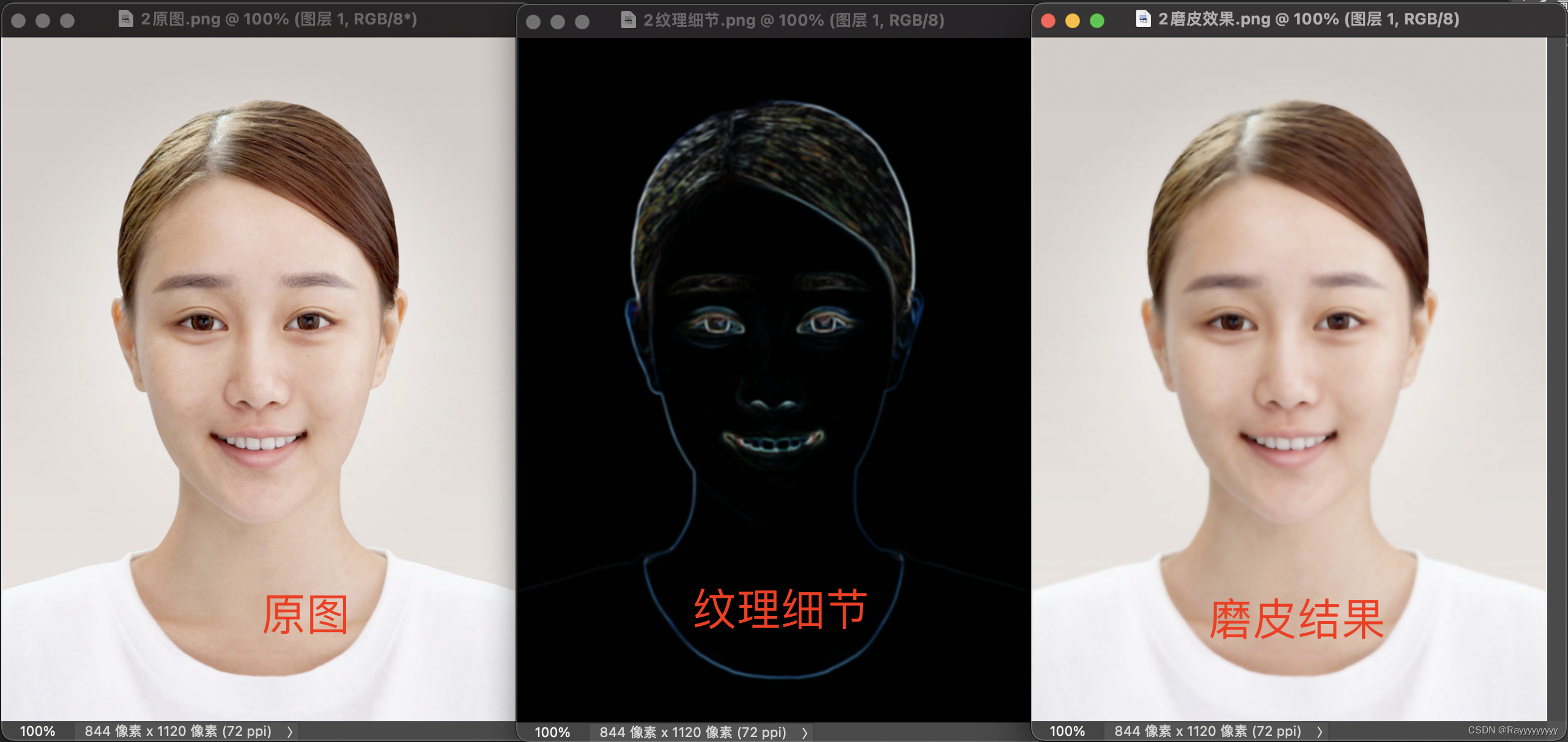
正则化参数eps=0.02
动态效果展示
- 1.固定模糊程度(0.5),修改正则化参数eps(变化范围 0~0.1)
- 2.固定正则化参数eps(0.05),修改模糊程度0~1