欢迎大家关注全网生信学习者系列:
- WX公zhong号:生信学习者
- Xiao hong书:生信学习者
- 知hu:生信学习者
- CDSN:生信学习者2
介绍
微生物数据具有一下的特点,这使得在做差异分析的时候需要考虑到更多的问题,
-
Sparsity
-
Compositional
-
Overdispersion
现在 **Nearing, Douglas et al. Nature Comm. Microbiome differential abundance methods produce different results across 38 datasets.**文章对常用的差异分析方法做了基准测试,本文讲把不同方法的核心计算代码记录下来。
作者这项工作的目标是比较一系列常见的差异分析(DA)方法在16S rRNA基因数据集上的表现。因此,在这项工作的大部分中,作者并不确切知道正确答案是什么:作者主要只能说哪些工具在性能上更相似于其他工具。然而,还包含了几项分析,以帮助评估这些工具在不同环境下来自同一数据集的假阳性率和一致性。
简单地说,该工作试图评估不同的微生物组差异丰度分析方法在多个数据集上的表现,并比较它们之间的相似性和一致性,同时尝试评估这些工具在不同数据集上产生假阳性结果的频率。
Sparsity
即使在同一环境中,不同样本的微生物出现概率或者丰度都是不一样的,大部分微生物丰度极低。又因为在测序仪的检测极限下,微生物丰度(相对或绝对丰度)为0的概率又极大增加了。除此之外,比对所使用的数据库大小也即是覆盖物种率也会对最终的微生物丰度表达谱有较大的影响。最后我们所获得的微生物丰度谱必然含有大量的零值,它有两种情况,一种是真实的零值,另一种是误差导致的零值。很多算法会针对这两个特性构建不同的处理零值策略。
零值数量的大小构成了微生物丰度谱稀疏性。在某次16s数据的OTU水平中,零值比例高达80%以上。Sparsity属性导致常用的数据分析方法如t-test/wilcox-test假设检验方法均不适合。为了解决sparsity对分析的影响,很多R包的方法如ANCOM的Zero划分,metagenomeSeq的ZIP/ZILN对Zero进行处理,处理后的矩阵再做如CLR等变换,CLR变换又是为了处理微生物数据另一个特点compositional (下一部分讲)。最后转换后的数据会服从常见的分布,也即是可以使用常见的如Wilcox/t-test之类(两分组)的方法做假设检验,需要说明的是ANCOM还会根据物种在样本内的显著性的差异比例区分差异物种,这也是为何ANCOM的稳健性的原因。
Compositional
Compositional的数据特性是服从simplex空间,简而言之是指:某个样本内所有微生物的加和是一个常数(可以是1也可以是10,100)。符合该属性的数据内部元素之间存在着相关关系,即某个元素的比例发生波动,必然引起其他元素比例的波动,但在实际的微生物环境中,这种关联关系可能是不存在的。为了解决compositional的问题,有人提出了使用各种normalization方法(比如上文提到的CLR: X i = l o g ( x i G e a m e t r i c M e a n ( X ) ) X_{i}=log(\frac{x_{i}}{GeametricMean(X)}) Xi=log(GeametricMean(X)xi),我暂时只熟悉这个方法)。
Compositional数据不服从欧式空间分布,在使用log-ratio transformation后,数据可以一一对应到真实的多维变量的空间,方便后续应用标准分析方法。
Overdispersion
Overdispersion的条件是 Variance >> mean,也就是说数据的方差要远远大于均值。常用的适合count matrix的Poisson分布是无法处理这样的数据的,因此现在很多方法都是用负二项分布去拟合数据。
总结
使用一张自己讲过的PPT总结一下。

差异分析方法
不同的差异分析方法识别到差异微生物可能会存在较大的区别,这是因为这些方法的原理是不一样的,但从微生物的数据特点而言,方法需要符合微生物数据特性。
ALDEx2
ALDEx2(ANOVA-Like Differential Expression 2)是一种用于微生物组数据差异分析的方法,它特别适用于处理组成数据(compositional data),这类数据的特点是在每个样本中各部分的总和为一个固定值,例如微生物群落中各物种的相对丰度之和为1。ALDEx2方法的核心原理包括以下几个步骤:
- 生成后验概率分布:首先,ALDEx2使用Dirichlet分布来模拟每个分类单元(如OTU或ASV)的读数计数的后验概率分布。这一步是基于微生物群落数据的组成特性,即数据点在高维空间中位于一个低维的简单形(simplex)上。
- 中心对数比变换(CLR):ALDEx2对原始计数数据进行中心对数比(Centered Log-Ratio)变换,这是一种适合组成数据的变换方法,可以消除数据的组成特性带来的影响,使得数据更适合常规的统计分析方法。
- 单变量统计检验:变换后的数据将用于单变量统计检验,如Welch’s t检验或秩和检验,以确定不同组之间各分类单元的丰度是否存在显著差异。
- 效应量估计:ALDEx2还计算效应量大小,这是衡量组间差异相对于组内变异的一个重要指标,有助于评估差异的生物学意义。
- 多重检验校正:在识别出显著差异的分类单元后,ALDEx2使用Benjamini-Hochberg方法进行多重检验校正,以控制假阳性率。
#### Script to Run ALDEX2 differential abundance

deps = c("ALDEx2")
for (dep in deps){
  if (dep %in% installed.packages()[,"Package"] == FALSE){
    if (!requireNamespace("BiocManager", quietly = TRUE))
      install.packages("BiocManager")

    BiocManager::install("ALDEx2")
  }
  library(dep, character.only = TRUE)
}

library(ALDEx2)

args <- commandArgs(trailingOnly = TRUE)


#test if there is an argument supply
if (length(args) <= 2) {
  stop("At least three arguments must be supplied", call.=FALSE)
}

con <- file(args[1])
file_1_line1 <- readLines(con,n=1)
close(con)

if(grepl("Constructed from biom file", file_1_line1)){
  ASV_table <- read.table(args[1], sep="\t", skip=1, header=T, row.names = 1,
                            comment.char = "", quote="", check.names = F)
}else{
  ASV_table <- read.table(args[1], sep="\t", header=T, row.names = 1,
                            comment.char = "", quote="", check.names = F)
}

groupings <- read.table(args[2], sep="\t", row.names = 1, header=T, comment.char = "", quote="", check.names = F)

#number of samples
sample_num <- length(colnames(ASV_table))
grouping_num <- length(rownames(groupings))

#check if the same number of samples are being input.
if(sample_num != grouping_num){
  message("The number of samples in the ASV table and the groupings table are unequal")
  message("Will remove any samples that are not found in either the ASV table or the groupings table")
}

#check if order of samples match up.
if(identical(colnames(ASV_table), rownames(groupings))==T){
  message("Groupings and ASV table are in the same order")
}else{
  rows_to_keep <- intersect(colnames(ASV_table), rownames(groupings))
  groupings <- groupings[rows_to_keep,,drop=F]
  ASV_table <- ASV_table[,rows_to_keep]
  if(identical(colnames(ASV_table), rownames(groupings))==T){
    message("Groupings table was re-arrange to be in the same order as the ASV table")
    message("A total of ", sample_num-length(colnames(ASV_table)), " from the ASV_table")
    message("A total of ", grouping_num-length(rownames(groupings)), " from the groupings table")
  }else{
    stop("Unable to match samples between the ASV table and groupings table")
  }
}

results <- aldex(reads = ASV_table,
                conditions = groupings[, 1],
                mc.samples = 128,
                test = "t",
                effect = TRUE,
                include.sample.summary = FALSE,
                verbose = T,
                denom = "all")

write.table(results, file=args[3], quote=FALSE, sep='\t', col.names = NA)


message("Results table saved to ", args[3])
ANCOM-II
ANCOM(Analysis of Composition of Microbiomes)是一种用于分析微生物组数据的统计方法,专门设计来识别和比较不同样本或处理组之间的微生物组成差异。其核心原理包括以下几个步骤:
- 数据聚合:首先,对数据进行预处理,去除低丰度的微生物分类单元(OTU/ASV),并对数据进行标准化或转换操作,将绝对丰度转换为相对丰度。
- 添加伪计数:由于ANCOM分析过程中需要使用对数变换,而相对丰度为0的分类群无法进行对数变换,因此需要添加一个小的正数作为伪计数,以解决这个问题。
- 计算特征差异:ANCOM使用W统计量来检测不同组之间的特征是否存在显著差异。W统计量的计算包括以下步骤:
- 对每个特征在所有样本中的相对丰度进行排序。
- 将样本分为目标组和参考组,通常情况下,目标组是研究者感兴趣的组别,而参考组是其他组别的合并。
- 计算目标组和参考组中每个特征的累积相对丰度,即从最低相对丰度的特征开始,逐渐累积到当前特征的相对丰度之和。
- 计算目标组和参考组中每个特征的平均累积相对丰度。
- 计算目标组和参考组之间的差异值,即目标组的平均累积相对丰度减去参考组的均累积相对丰度。
- 计算每个特征的W统计量,即将差异值除以其标准差。W统计量的绝对值大于1.96通常被认为是显著差异的特征。
- 结果解读:ANCOM的结果通常包括火山图和统计表格,火山图展示了W统计量与中心对数比例(CLR)变换后的数据,而统计表格列出了差异显著的特征及其相关信息。
ANCOM的优点包括能够处理稀疏数据、保持较低的误报率以及对异常值具有鲁棒性。然而,它也存在一些限制,例如对数据的分布假设敏感,对样本数目和特征维度的要求较高
deps = c("exactRankTests", "nlme", "dplyr", "ggplot2", "compositions")
for (dep in deps){
  if (dep %in% installed.packages()[,"Package"] == FALSE){
    install.packages(dep)
  }
  library(dep, character.only = TRUE)
}

#args[4] will contain path for the ancom code


args <- commandArgs(trailingOnly = TRUE)

if (length(args) <= 3) {
  stop("At least three arguments must be supplied", call.=FALSE)
}

source(args[[4]])

con <- file(args[1])
file_1_line1 <- readLines(con,n=1)
close(con)

if(grepl("Constructed from biom file", file_1_line1)){
  ASV_table <- read.table(args[1], sep="\t", skip=1, header=T, row.names = 1,
                          comment.char = "", quote="", check.names = F)
}else{
  ASV_table <- read.table(args[1], sep="\t", header=T, row.names = 1,
                          comment.char = "", quote="", check.names = F)
}

groupings <- read.table(args[2], sep="\t", row.names = 1, header=T, comment.char = "", quote="", check.names = F)

#number of samples
sample_num <- length(colnames(ASV_table))
grouping_num <- length(rownames(groupings))

if(sample_num != grouping_num){
  message("The number of samples in the ASV table and the groupings table are unequal")
  message("Will remove any samples that are not found in either the ASV table or the groupings table")
}

if(identical(colnames(ASV_table), rownames(groupings))==T){
  message("Groupings and ASV table are in the same order")
}else{
  rows_to_keep <- intersect(colnames(ASV_table), rownames(groupings))
  groupings <- groupings[rows_to_keep,,drop=F]
  ASV_table <- ASV_table[,rows_to_keep]
  if(identical(colnames(ASV_table), rownames(groupings))==T){
    message("Groupings table was re-arrange to be in the same order as the ASV table")
    message("A total of ", sample_num-length(colnames(ASV_table)), " from the ASV_table")
    message("A total of ", grouping_num-length(rownames(groupings)), " from the groupings table")
  }else{
    stop("Unable to match samples between the ASV table and groupings table")
  }
}

groupings$Sample <- rownames(groupings)

prepro <- feature_table_pre_process(feature_table = ASV_table,
                                    meta_data = groupings,
                                    sample_var = 'Sample',
                                    group_var = NULL,
                                    out_cut = 0.05,
                                    zero_cut = 0.90,
                                    lib_cut = 1000,
                                    neg_lb=FALSE)

feature_table <- prepro$feature_table
metadata <- prepro$meta_data
struc_zero <- prepro$structure_zeros

#run ancom
main_var <- colnames(groupings)[1]
p_adj_method = "BH"
alpha=0.05
adj_formula=NULL
rand_formula=NULL
res <- ANCOM(feature_table = feature_table,
             meta_data = metadata,
             struc_zero = struc_zero,
             main_var = main_var,
             p_adj_method = p_adj_method,
             alpha=alpha,
             adj_formula = adj_formula,
             rand_formula = rand_formula)


write.table(res$out, file=args[3], quote=FALSE, sep="\t", col.names = NA)
Corncob
Corncob 是一种用于微生物组数据分析的R包,它专门用于对微生物相对丰度进行建模并测试协变量对相对丰度的影响。其核心原理包括以下几个方面:
- 相对丰度建模:Corncob 通过统计模型来分析微生物的相对丰度数据,考虑到数据的组成性特征,即样本中各微生物的相对丰度总和为1。
- β-二项式分布:Corncob 假设微生物的计数数据遵循β-二项式分布,这种分布可以更好地描述微生物组数据中的离散性和过度离散现象。
- 协变量效应测试:Corncob 允许研究者测试一个或多个协变量对微生物相对丰度的影响,这可以通过Wald检验等统计方法来实现。
- 多重假设检验校正:在分析过程中,Corncob 会对多重比较问题进行校正,以控制第一类错误率,常用的校正方法包括Benjamini-Hochberg (BH) 方法。
- 模型拟合与假设检验:Corncob 进行模型拟合并对模型参数进行估计,然后通过假设检验确定特定微生物分类群的相对丰度是否存在显著差异。
- 稀疏性和零膨胀数据处理:Corncob 还考虑到了微生物组数据的稀疏性,即许多微生物在多数样本中可能未被检测到,以及零膨胀问题,即存在大量零计数的情况。
#### Run Corncob

library(corncob)
library(phyloseq)

#install corncob if its not installed.
deps = c("corncob")
for (dep in deps){
  if (dep %in% installed.packages()[,"Package"] == FALSE){
    if(dep=="corncob"){
      devtools::install_github("bryandmartin/corncob")
    }
    else
      if (!requireNamespace("BiocManager", quietly = TRUE))
        install.packages("BiocManager")

    BiocManager::install("phyloseq")
  }
  library(dep, character.only = TRUE)
}


args <- commandArgs(trailingOnly = TRUE)

if (length(args) <= 2) {
  stop("At least three arguments must be supplied", call.=FALSE)
}

con <- file(args[1])
file_1_line1 <- readLines(con,n=1)
close(con)

if(grepl("Constructed from biom file", file_1_line1)){
  ASV_table <- read.table(args[1], sep="\t", skip=1, header=T, row.names = 1,
                          comment.char = "", quote="", check.names = F)
}else{
  ASV_table <- read.table(args[1], sep="\t", header=T, row.names = 1,
                          comment.char = "", quote="", check.names = F)
}

groupings <- read.table(args[2], sep="\t", row.names = 1, header=T, comment.char = "", quote="", check.names = F)

#number of samples
sample_num <- length(colnames(ASV_table))
grouping_num <- length(rownames(groupings))

#check if the same number of samples are being input.
if(sample_num != grouping_num){
  message("The number of samples in the ASV table and the groupings table are unequal")
  message("Will remove any samples that are not found in either the ASV table or the groupings table")
}

#check if order of samples match up.
if(identical(colnames(ASV_table), rownames(groupings))==T){
  message("Groupings and ASV table are in the same order")
}else{
  rows_to_keep <- intersect(colnames(ASV_table), rownames(groupings))
  groupings <- groupings[rows_to_keep,,drop=F]
  ASV_table <- ASV_table[,rows_to_keep]
  if(identical(colnames(ASV_table), rownames(groupings))==T){
    message("Groupings table was re-arrange to be in the same order as the ASV table")
    message("A total of ", sample_num-length(colnames(ASV_table)), " from the ASV_table")
    message("A total of ", grouping_num-length(rownames(groupings)), " from the groupings table")
  }else{
    stop("Unable to match samples between the ASV table and groupings table")
  }
}

#run corncob
#put data into phyloseq object.
colnames(groupings)
colnames(groupings)[1] <- "places"

OTU <- phyloseq::otu_table(ASV_table, taxa_are_rows = T)
sampledata <- phyloseq::sample_data(groupings, errorIfNULL = T)
phylo <- phyloseq::merge_phyloseq(OTU, sampledata)

my_formula <- as.formula(paste("~","places",sep=" ", collapse = ""))
my_formula
results <- corncob::differentialTest(formula= my_formula,
                                     phi.formula = my_formula,
                                     phi.formula_null = my_formula,
                                     formula_null = ~ 1,
                                     test="Wald", data=phylo,
                                     boot=F,
                                     fdr_cutoff = 0.05)


write.table(results$p_fdr, file=args[[3]], sep="\t", col.names = NA, quote=F)
write.table(results$p, file=paste0(args[[3]], "_uncor", sep=""), sep="\t", col.names = NA, quote=F)
DESeq2
DESeq2是一种用于微生物组数据差异分析的统计方法,特别适用于处理计数数据,如RNA-seq数据或微生物组的OTU(操作分类单元)计数。DESeq2的核心原理包括以下几个关键步骤:
- 数据标准化:DESeq2首先对原始的计数数据进行标准化,以校正样本间的测序深度差异。这是通过计算大小因子(size factors)实现的,每个样本的大小因子乘以其总计数,以调整测序深度。
- 离散度估计:DESeq2估计每个特征(如OTU或基因)的离散度,即数据的变异程度。离散度是负二项分布的一个参数,用于描述数据的过度离散现象。
- 经验贝叶斯收缩:DESeq2使用经验贝叶斯方法对离散度进行收缩,即利用所有特征的离散度估计来改进个别特征的离散度估计,这有助于提高统计估计的稳定性。
- 负二项分布建模:DESeq2假设计数数据遵循负二项分布,该分布是处理计数数据的常用分布,特别适用于处理微生物组数据中的零膨胀现象。
- 设计公式:DESeq2通过设计公式来考虑实验设计,包括处理效应、批次效应和其他协变量,从而允许研究者评估特定条件下的微生物差异丰度。
- 假设检验:DESeq2使用统计检验来确定不同样本组之间特定微生物的丰度是否存在显著差异。这通常涉及比较零假设(两组间无差异)和备择假设(两组间有差异)。
- 多重检验校正:由于微生物组数据涉及大量多重比较,DESeq2使用Benjamini-Hochberg方法进行多重检验校正,以控制假发现率(FDR)。
- 结果解释:DESeq2提供了丰富的结果输出,包括P值、校正后的P值、对数倍数变化(log2 fold change)等,这些结果可以帮助研究者识别和解释数据中的生物学意义。
#Run_DeSeq2

deps = c("DESeq2")
for (dep in deps){
  if (dep %in% installed.packages()[,"Package"] == FALSE){
    if (!requireNamespace("BiocManager", quietly = TRUE))
      install.packages("BiocManager")

    BiocManager::install("DESeq2")
  }
  library(dep, character.only = TRUE)
}

library(DESeq2)


args <- commandArgs(trailingOnly = TRUE)
#test if there is an argument supply
if (length(args) <= 2) {
  stop("At least three arguments must be supplied", call.=FALSE)
}

con <- file(args[1])
file_1_line1 <- readLines(con,n=1)
close(con)

if(grepl("Constructed from biom file", file_1_line1)){
  ASV_table <- read.table(args[1], sep="\t", skip=1, header=T, row.names = 1,
                          comment.char = "", quote="", check.names = F)
}else{
  ASV_table <- read.table(args[1], sep="\t", header=T, row.names = 1,
                          comment.char = "", quote="", check.names = F)
}

groupings <- read.table(args[2], sep="\t", row.names = 1, header=T, comment.char = "", quote="", check.names = F)

#number of samples
sample_num <- length(colnames(ASV_table))
grouping_num <- length(rownames(groupings))

#check if the same number of samples are being input.
if(sample_num != grouping_num){
  message("The number of samples in the ASV table and the groupings table are unequal")
  message("Will remove any samples that are not found in either the ASV table or the groupings table")
}

#check if order of samples match up.
if(identical(colnames(ASV_table), rownames(groupings))==T){
  message("Groupings and ASV table are in the same order")
}else{
  rows_to_keep <- intersect(colnames(ASV_table), rownames(groupings))
  groupings <- groupings[rows_to_keep,,drop=F]
  ASV_table <- ASV_table[,rows_to_keep]
  if(identical(colnames(ASV_table), rownames(groupings))==T){
    message("Groupings table was re-arrange to be in the same order as the ASV table")
    message("A total of ", sample_num-length(colnames(ASV_table)), " from the ASV_table")
    message("A total of ", grouping_num-length(rownames(groupings)), " from the groupings table")
  }else{
    stop("Unable to match samples between the ASV table and groupings table")
  }
}

colnames(groupings)[1] <- "Groupings"
#Run Deseq2

dds <- DESeq2::DESeqDataSetFromMatrix(countData = ASV_table,
                                      colData=groupings,
                                      design = ~ Groupings)
dds_res <- DESeq2::DESeq(dds, sfType = "poscounts")

res <- results(dds_res, tidy=T, format="DataFrame")

rownames(res) <- res$row
res <- res[,-1]

write.table(res, file=args[3], quote=FALSE, sep="\t", col.names = NA)

message("Results written to ", args[3])
edgeR
EdgeR(Empirical Analysis of Digital Gene Expression in R)是一种用于分析计数数据的统计方法,特别适用于微生物组学、转录组学和其他高通量测序技术产生的数据。EdgeR的核心原理包括以下几个关键步骤:
- 数据标准化:EdgeR通过计算标准化因子(Normalization Factors)来调整不同样本的测序深度或库大小,确保比较的公平性。
- 离散度估计:EdgeR估计每个基因或OTU的离散度(Dispersion),这是衡量数据变异程度的一个参数,对于后续的统计检验至关重要。
- 负二项分布建模:EdgeR假设数据遵循负二项分布,这是一种常用于计数数据的分布模型,可以处理数据的过度离散现象。
- 经验贝叶斯收缩:EdgeR使用经验贝叶斯方法对离散度进行收缩(Shrinkage),通过借用全局信息来提高对每个基因或OTU离散度估计的准确性。
- 设计矩阵:EdgeR通过设计矩阵(Design Matrix)来表示实验设计,包括处理效应、时间效应、批次效应等,允许研究者评估不同条件下的基因或OTU表达差异。
- 统计检验:EdgeR进行似然比检验(Likelihood Ratio Test, LRT)或精确检验(Exact Test),以确定不同样本组之间特定基因或OTU的表达是否存在显著差异。
- 多重检验校正:EdgeR使用多种方法进行多重检验校正,如Benjamini-Hochberg(BH)方法,以控制假发现率(FDR)。
- 结果解释:EdgeR提供了丰富的结果输出,包括P值、校正后的P值、对数倍数变化(Log Fold Change, LFC)等,帮助研究者识别和解释数据中的生物学变化。
deps = c("edgeR", "phyloseq")
for (dep in deps){
  if (dep %in% installed.packages()[,"Package"] == FALSE){
    if (!requireNamespace("BiocManager", quietly = TRUE))
      install.packages("BiocManager")

    BiocManager::install(deps)
  }
  library(dep, character.only = TRUE)
}

### Taken from phyloseq authors at: https://joey711.github.io/phyloseq-extensions/edgeR.html
phyloseq_to_edgeR = function(physeq, group, method="RLE", ...){
  require("edgeR")
  require("phyloseq")
  # Enforce orientation.
  if( !taxa_are_rows(physeq) ){ physeq <- t(physeq) }
  x = as(otu_table(physeq), "matrix")
  # Add one to protect against overflow, log(0) issues.
  x = x + 1
  # Check `group` argument
  if( identical(all.equal(length(group), 1), TRUE) & nsamples(physeq) > 1 ){
    # Assume that group was a sample variable name (must be categorical)
    group = get_variable(physeq, group)
  }
  # Define gene annotations (`genes`) as tax_table
  taxonomy = tax_table(physeq, errorIfNULL=FALSE)
  if( !is.null(taxonomy) ){
    taxonomy = data.frame(as(taxonomy, "matrix"))
  }
  # Now turn into a DGEList
  y = DGEList(counts=x, group=group, genes=taxonomy, remove.zeros = TRUE, ...)
  # Calculate the normalization factors
  z = calcNormFactors(y, method=method)
  # Check for division by zero inside `calcNormFactors`
  if( !all(is.finite(z$samples$norm.factors)) ){
    stop("Something wrong with edgeR::calcNormFactors on this data,
         non-finite $norm.factors, consider changing `method` argument")
  }
  # Estimate dispersions
  return(estimateTagwiseDisp(estimateCommonDisp(z)))
}


args <- commandArgs(trailingOnly = TRUE)
#test if there is an argument supply
if (length(args) <= 2) {
  stop("At least three arguments must be supplied", call.=FALSE)
}

con <- file(args[1])
file_1_line1 <- readLines(con,n=1)
close(con)

if(grepl("Constructed from biom file", file_1_line1)){
  ASV_table <- read.table(args[1], sep="\t", skip=1, header=T, row.names = 1,
                          comment.char = "", quote="", check.names = F)
}else{
  ASV_table <- read.table(args[1], sep="\t", header=T, row.names = 1,
                          comment.char = "", quote="", check.names = F)
}

groupings <- read.table(args[2], sep="\t", row.names = 1, header=T, comment.char = "", quote="", check.names = F)

#number of samples
sample_num <- length(colnames(ASV_table))
grouping_num <- length(rownames(groupings))

#check if the same number of samples are being input.
if(sample_num != grouping_num){
  message("The number of samples in the ASV table and the groupings table are unequal")
  message("Will remove any samples that are not found in either the ASV table or the groupings table")
}

#check if order of samples match up.
if(identical(colnames(ASV_table), rownames(groupings))==T){
  message("Groupings and ASV table are in the same order")
}else{
  rows_to_keep <- intersect(colnames(ASV_table), rownames(groupings))
  groupings <- groupings[rows_to_keep,,drop=F]
  ASV_table <- ASV_table[,rows_to_keep]
  if(identical(colnames(ASV_table), rownames(groupings))==T){
    message("Groupings table was re-arrange to be in the same order as the ASV table")
    message("A total of ", sample_num-length(colnames(ASV_table)), " from the ASV_table")
    message("A total of ", grouping_num-length(rownames(groupings)), " from the groupings table")
  }else{
    stop("Unable to match samples between the ASV table and groupings table")
  }
}

OTU <- phyloseq::otu_table(ASV_table, taxa_are_rows = T)
sampledata <- phyloseq::sample_data(groupings, errorIfNULL = T)
phylo <- phyloseq::merge_phyloseq(OTU, sampledata)

test <- phyloseq_to_edgeR(physeq = phylo, group=colnames(groupings)[1])

et = exactTest(test)

tt = topTags(et, n=nrow(test$table), adjust.method="fdr", sort.by="PValue")
res <- tt@.Data[[1]]

write.table(res, file=args[3], quote=F, sep="\t", col.names = NA)
Limma-Voom-TMM
Limma-Voom-TMM(Trimmed Mean of M-values)是一种用于微生物组数据差异分析的方法,它结合了limma、voom和TMM(Trimmed Mean of M-values)技术的优势,以处理和分析来自高通量测序技术(如RNA-seq)的数据。下面是Limma-Voom-TMM方法的基本原理:
- 数据预处理:首先,使用limma包中的预处理功能对原始的测序数据进行质量控制和标准化处理。
- TMM标准化:TMM是一种用于RNA-seq数据的标准化方法,它通过计算所有基因的几何平均表达值,然后对每个基因的表达值进行缩放,以校正样本间的测序深度差异。
- voom转换:voom是一种用于将计数数据转换为适合线性模型分析的格式的方法。它通过对数据进行对数变换和中心化处理,将原始的计数数据转换为相对于某个参照样本的比例,从而减少数据的离散性。
- 线性模型:Limma-Voom方法使用线性模型来分析数据,这种模型可以包括多个协变量和批次效应,以评估不同样本组之间的基因表达差异。
- 经验贝叶斯估计:Limma-Voom方法使用经验贝叶斯统计来估计基因表达的离散度,这有助于提高对基因表达变化的检测灵敏度。
- 统计检验:在模型拟合之后,Limma-Voom进行统计检验来确定基因表达是否存在显著差异。这通常涉及到似然比检验(LRT)或t检验。
- 多重检验校正:由于同时测试多个基因,Limma-Voom使用多重检验校正方法(如Benjamini-Hochberg方法)来控制假发现率(FDR)。
- 结果解释:最终,Limma-Voom提供了一系列结果,包括P值、校正后的P值、对数倍数变化(Log Fold Change, LFC)等,这些结果可以帮助研究者识别差异表达的基因或微生物类群。
deps = c("edgeR")
for (dep in deps){
  if (dep %in% installed.packages()[,"Package"] == FALSE){
    if (!requireNamespace("BiocManager", quietly = TRUE))
      install.packages("BiocManager")

    BiocManager::install(deps)
  }
  library(dep, character.only = TRUE)
}


args <- commandArgs(trailingOnly = TRUE)
#test if there is an argument supply
if (length(args) <= 2) {
  stop("At least three arguments must be supplied", call.=FALSE)
}

con <- file(args[1])
file_1_line1 <- readLines(con,n=1)
close(con)

if(grepl("Constructed from biom file", file_1_line1)){
  ASV_table <- read.table(args[1], sep="\t", skip=1, header=T, row.names = 1,
                          comment.char = "", quote="", check.names = F)
}else{
  ASV_table <- read.table(args[1], sep="\t", header=T, row.names = 1,
                          comment.char = "", quote="", check.names = F)
}

groupings <- read.table(args[2], sep="\t", row.names = 1, header=T, comment.char = "", quote="", check.names = F)

#number of samples
sample_num <- length(colnames(ASV_table))
grouping_num <- length(rownames(groupings))

#check if the same number of samples are being input.
if(sample_num != grouping_num){
  message("The number of samples in the ASV table and the groupings table are unequal")
  message("Will remove any samples that are not found in either the ASV table or the groupings table")
}

#check if order of samples match up.
if(identical(colnames(ASV_table), rownames(groupings))==T){
  message("Groupings and ASV table are in the same order")
}else{
  rows_to_keep <- intersect(colnames(ASV_table), rownames(groupings))
  groupings <- groupings[rows_to_keep,,drop=F]
  ASV_table <- ASV_table[,rows_to_keep]
  if(identical(colnames(ASV_table), rownames(groupings))==T){
    message("Groupings table was re-arrange to be in the same order as the ASV table")
    message("A total of ", sample_num-length(colnames(ASV_table)), " from the ASV_table")
    message("A total of ", grouping_num-length(rownames(groupings)), " from the groupings table")
  }else{
    stop("Unable to match samples between the ASV table and groupings table")
  }
}

DGE_LIST <- DGEList(ASV_table)
### do normalization
### Reference sample will be the sample with the highest read depth

### check if upper quartile method works for selecting reference
Upper_Quartile_norm_test <- calcNormFactors(DGE_LIST, method="upperquartile")

summary_upper_quartile <- summary(Upper_Quartile_norm_test$samples$norm.factors)[3]
if(is.na(summary_upper_quartile) | is.infinite(summary_upper_quartile)){
  message("Upper Quartile reference selection failed will use find sample with largest sqrt(read_depth) to use as reference")
  Ref_col <- which.max(colSums(sqrt(ASV_table)))
  DGE_LIST_Norm <- calcNormFactors(DGE_LIST, method = "TMM", refColumn = Ref_col)
  fileConn<-file(args[[4]])
  writeLines(c("Used max square root read depth to determine reference sample"), fileConn)
  close(fileConn)

}else{
  DGE_LIST_Norm <- calcNormFactors(DGE_LIST, method="TMM")
}

## make matrix for testing
colnames(groupings) <- c("comparison")
mm <- model.matrix(~comparison, groupings)

voomvoom <- voom(DGE_LIST_Norm, mm, plot=F)

fit <- lmFit(voomvoom,mm)
fit <- eBayes(fit)
res <- topTable(fit, coef=2, n=nrow(DGE_LIST_Norm), sort.by="none")
write.table(res, file=args[3], quote=F, sep="\t", col.names = NA)
Limma-Voom-TMMwsp
Limma-Voom-TMMwsp(Trimmed Mean of M-values with Singleton Pairing)是一种用于处理和分析微生物组数据的差异分析方法,它结合了几种不同的统计技术来提高分析的准确性和可靠性。下面是Limma-Voom-TMMwsp方法的基本原理:
- 数据预处理:首先,对原始的测序数据进行质量控制和预处理操作,包括去除低质量的读段、过滤掉可能的污染物等。
- TMMwsp标准化:TMMwsp是一种标准化方法,用于校正不同样本之间的测序深度差异。它通过对每个样本的计数数据应用TMM方法,并在计算中考虑单例配对(singleton pairing),以减少由于样本间测序深度不同带来的偏差。
- voom转换:voom是一种转换方法,用于将原始的计数数据转换为适合线性模型分析的格式。voom通过对数据进行对数变换,并根据样本之间的差异来估计每个基因或OTU的准确差异度量。
- 线性模型:Limma-Voom方法使用线性模型来分析数据,这种模型可以包括多个协变量和批次效应,以评估不同样本组之间的基因或OTU表达差异。
- 经验贝叶斯估计:Limma-Voom方法使用经验贝叶斯统计来估计基因或OTU表达的离散度,这有助于提高对基因或OTU表达变化的检测灵敏度。
- 统计检验:在模型拟合之后,Limma-Voom进行统计检验来确定基因或OTU表达是否存在显著差异。这通常涉及到似然比检验(LRT)或t检验。
- 多重检验校正:由于同时测试多个基因或OTU,Limma-Voom使用多重检验校正方法(如Benjamini-Hochberg方法)来控制假发现率(FDR)。
- 结果解释:最终,Limma-Voom提供了一系列结果,包括P值、校正后的P值、对数倍数变化(Log Fold Change, LFC)等,这些结果可以帮助研究者识别差异表达的基因或微生物类群。
deps = c("edgeR")
for (dep in deps){
  if (dep %in% installed.packages()[,"Package"] == FALSE){
    if (!requireNamespace("BiocManager", quietly = TRUE))
      install.packages("BiocManager")

    BiocManager::install(deps)
  }
  library(dep, character.only = TRUE)
}


args <- commandArgs(trailingOnly = TRUE)
#test if there is an argument supply
if (length(args) <= 2) {
  stop("At least three arguments must be supplied", call.=FALSE)
}

con <- file(args[1])
file_1_line1 <- readLines(con,n=1)
close(con)

if(grepl("Constructed from biom file", file_1_line1)){
  ASV_table <- read.table(args[1], sep="\t", skip=1, header=T, row.names = 1,
                          comment.char = "", quote="", check.names = F)
}else{
  ASV_table <- read.table(args[1], sep="\t", header=T, row.names = 1,
                          comment.char = "", quote="", check.names = F)
}

groupings <- read.table(args[2], sep="\t", row.names = 1, header=T, comment.char = "", quote="", check.names = F)

#number of samples
sample_num <- length(colnames(ASV_table))
grouping_num <- length(rownames(groupings))

#check if the same number of samples are being input.
if(sample_num != grouping_num){
  message("The number of samples in the ASV table and the groupings table are unequal")
  message("Will remove any samples that are not found in either the ASV table or the groupings table")
}

#check if order of samples match up.
if(identical(colnames(ASV_table), rownames(groupings))==T){
  message("Groupings and ASV table are in the same order")
}else{
  rows_to_keep <- intersect(colnames(ASV_table), rownames(groupings))
  groupings <- groupings[rows_to_keep,,drop=F]
  ASV_table <- ASV_table[,rows_to_keep]
  if(identical(colnames(ASV_table), rownames(groupings))==T){
    message("Groupings table was re-arrange to be in the same order as the ASV table")
    message("A total of ", sample_num-length(colnames(ASV_table)), " from the ASV_table")
    message("A total of ", grouping_num-length(rownames(groupings)), " from the groupings table")
  }else{
    stop("Unable to match samples between the ASV table and groupings table")
  }
}

DGE_LIST <- DGEList(ASV_table)
### do normalization
### Reference sample will be the sample with the highest read depth

### check if upper quartile method works for selecting reference
Upper_Quartile_norm_test <- calcNormFactors(DGE_LIST, method="upperquartile")

summary_upper_quartile <- summary(Upper_Quartile_norm_test$samples$norm.factors)[3]
if(is.na(summary_upper_quartile) | is.infinite(summary_upper_quartile)){
  message("Upper Quartile reference selection failed will use find sample with largest sqrt(read_depth) to use as reference")
  Ref_col <- which.max(colSums(sqrt(ASV_table)))
  DGE_LIST_Norm <- calcNormFactors(DGE_LIST, method = "TMMwsp", refColumn = Ref_col)
  fileConn<-file(args[[4]])
  writeLines(c("Used max square root read depth to determine reference sample"), fileConn)
  close(fileConn)
}else{
  DGE_LIST_Norm <- calcNormFactors(DGE_LIST, method="TMMwsp")
}

## make matrix for testing
colnames(groupings) <- c("comparison")
mm <- model.matrix(~comparison, groupings)

voomvoom <- voom(DGE_LIST_Norm, mm, plot=F)

fit <- lmFit(voomvoom,mm)
fit <- eBayes(fit)
res <- topTable(fit, coef=2, n=nrow(DGE_LIST_Norm), sort.by="none")
write.table(res, file=args[3], quote=F, sep="\t", col.names = NA)
Maaslin2
MaAsLin2是一种用于微生物组数据差异分析的统计方法,它专门设计用来处理微生物组数据的复杂性,包括噪声、稀疏性(零膨胀)、高维度、极端非正态分布以及通常以计数或组成性测量的形式出现的数据。以下是MaAsLin2方法的基本原理:
- 多变量统计框架:MaAsLin2(Microbiome Multivariable Associations with Linear Models)使用广义线性和混合模型来适应各种现代流行病学研究设计,包括横截面和纵向研究。
- 数据预处理:MaAsLin2提供了预处理模块,用于处理元数据和微生物特征中的缺失值、未知数据值和异常值。
- 归一化和转换:MaAsLin2可以对微生物测量结果进行归一化和转换,以解决样本中可变的覆盖深度。
- 特征标准化:可选择执行特征标准化,并使用元数据的子集或完整补充来模拟生成的质量控制微生物特征。
- 多变量模型:MaAsLin2使用各种可能的多变量模型之一为每个特征的每个元数据关联定义p值。
- 重复测量的处理:在存在重复测量的情况下,MaAsLin2通过在混合模型范式中适当地模拟对象内(或环境)相关来识别协变量相关的微生物特征,同时还通过指定对象间随机效应来解释个体变异在模型中。
- 统计检验:MaAsLin2可以识别每个单独特征与元数据对之间的关联,促进特征方面的协变量调整,并提高转化和基本生物学应用的可解释性。
- 结果校正:MaAsLin2还提供多重检验校正功能,以控制第一类错误率。
if(!requireNamespace("BiocManager", quietly = TRUE))
  install.packages("BiocManager")
#BiocManager::install("Maaslin2")

args <- commandArgs(trailingOnly = TRUE)

if (length(args) <= 2) {
  stop("At least three arguments must be supplied", call.=FALSE)
}


con <- file(args[1])
file_1_line1 <- readLines(con,n=1)
close(con)

if(grepl("Constructed from biom file", file_1_line1)){
  ASV_table <- read.table(args[1], sep="\t", skip=1, header=T, row.names = 1,
                          comment.char = "", quote="", check.names = F)
}else{
  ASV_table <- read.table(args[1], sep="\t", header=T, row.names = 1,
                          comment.char = "", quote="", check.names = F)
}
groupings <- read.table(args[2], sep="\t", row.names = 1, header=T, comment.char = "", quote="", check.names = F)

#number of samples
sample_num <- length(colnames(ASV_table))
grouping_num <- length(rownames(groupings))

if(sample_num != grouping_num){
  message("The number of samples in the ASV table and the groupings table are unequal")
  message("Will remove any samples that are not found in either the ASV table or the groupings table")
}

if(identical(colnames(ASV_table), rownames(groupings))==T){
  message("Groupings and ASV table are in the same order")
}else{
  rows_to_keep <- intersect(colnames(ASV_table), rownames(groupings))
  groupings <- groupings[rows_to_keep,,drop=F]
  ASV_table <- ASV_table[,rows_to_keep]
  if(identical(colnames(ASV_table), rownames(groupings))==T){
    message("Groupings table was re-arrange to be in the same order as the ASV table")
    message("A total of ", sample_num-length(colnames(ASV_table)), " from the ASV_table")
    message("A total of ", grouping_num-length(rownames(groupings)), " from the groupings table")
  }else{
    stop("Unable to match samples between the ASV table and groupings table")
  }
}


library(Maaslin2)


ASV_table <- data.frame(t(ASV_table), check.rows = F, check.names = F, stringsAsFactors = F)


fit_data <- Maaslin2(
  ASV_table, groupings,args[3], transform = "AST",
  fixed_effects = c(colnames(groupings[1])),
  standardize = FALSE, plot_heatmap = F, plot_scatter = F)
metagenomeSeq
metagenomeSeq是一种用于分析微生物组测序数据的统计学方法,它可以帮助研究人员发现不同条件下微生物组的差异丰度。以下是metagenomeSeq方法的基本原理:
- 数据预处理:metagenomeSeq首先对原始的测序数据进行质量控制和预处理,以确保数据的准确性和可靠性。
- 归一化:对测序数据进行归一化处理,以校正样本间的测序深度差异,确保不同样本间的比较是公平的。
- 统计模型:metagenomeSeq使用统计模型来分析数据,尤其是针对组成性数据的模型,比如零膨胀模型或负二项分布模型,这些模型可以处理微生物组数据的离散性和零膨胀问题。
- 差异丰度分析:metagenomeSeq确定在两个或多个组之间具有差异丰度的特征(如OTU、物种等),通过比较它们的相对丰度来识别差异。
- 多重检验校正:由于同时测试多个特征,metagenomeSeq使用多重检验校正方法(如Benjamini-Hochberg方法)来控制假发现率(FDR)。
- 结果解释:metagenomeSeq提供了丰富的结果输出,包括P值、校正后的P值、对数倍数变化(Log Fold Change, LFC)等,这些结果可以帮助研究者识别和解释数据中的生物学意义。
deps = c("metagenomeSeq")
for (dep in deps){
  if (dep %in% installed.packages()[,"Package"] == FALSE){
    if (!requireNamespace("BiocManager", quietly = TRUE))
      install.packages("BiocManager")

    BiocManager::install(deps)
  }
  library(dep, character.only = TRUE)
}

args <- commandArgs(trailingOnly = TRUE)
#test if there is an argument supply
if (length(args) <= 2) {
  stop("At least three arguments must be supplied", call.=FALSE)
}

con <- file(args[1])
file_1_line1 <- readLines(con,n=1)
close(con)

if(grepl("Constructed from biom file", file_1_line1)){
  ASV_table <- read.table(args[1], sep="\t", skip=1, header=T, row.names = 1,
                          comment.char = "", quote="", check.names = F)
}else{
  ASV_table <- read.table(args[1], sep="\t", header=T, row.names = 1,
                          comment.char = "", quote="", check.names = F)
}

groupings <- read.table(args[2], sep="\t", row.names = 1, header=T, comment.char = "", quote="", check.names = F)

#number of samples
sample_num <- length(colnames(ASV_table))
grouping_num <- length(rownames(groupings))

#check if the same number of samples are being input.
if(sample_num != grouping_num){
  message("The number of samples in the ASV table and the groupings table are unequal")
  message("Will remove any samples that are not found in either the ASV table or the groupings table")
}

#check if order of samples match up.
if(identical(colnames(ASV_table), rownames(groupings))==T){
  message("Groupings and ASV table are in the same order")
}else{
  rows_to_keep <- intersect(colnames(ASV_table), rownames(groupings))
  groupings <- groupings[rows_to_keep,,drop=F]
  ASV_table <- ASV_table[,rows_to_keep]
  if(identical(colnames(ASV_table), rownames(groupings))==T){
    message("Groupings table was re-arrange to be in the same order as the ASV table")
    message("A total of ", sample_num-length(colnames(ASV_table)), " from the ASV_table")
    message("A total of ", grouping_num-length(rownames(groupings)), " from the groupings table")
  }else{
    stop("Unable to match samples between the ASV table and groupings table")
  }
}

data_list <- list()
data_list[["counts"]] <- ASV_table
data_list[["taxa"]] <- rownames(ASV_table)

pheno <- AnnotatedDataFrame(groupings)
pheno
counts <- AnnotatedDataFrame(ASV_table)
feature_data <- data.frame("ASV"=rownames(ASV_table),
                           "ASV2"=rownames(ASV_table))
feature_data <- AnnotatedDataFrame(feature_data)
rownames(feature_data) <- feature_data@data$ASV


test_obj <- newMRexperiment(counts = data_list$counts, phenoData = pheno, featureData = feature_data)

p <- cumNormStat(test_obj, pFlag = T)
p

test_obj_norm <- cumNorm(test_obj, p=p)

fromula <- as.formula(paste(~1, colnames(groupings)[1], sep=" + "))
pd <- pData(test_obj_norm)
mod <- model.matrix(fromula, data=pd)
regres <- fitFeatureModel(test_obj_norm, mod)

res_table <- MRfulltable(regres, number = length(rownames(ASV_table)))

write.table(res_table, file=args[3], quote=F, sep="\t", col.names = NA)
T-test-rare
T-test-rarefaction是一种用于微生物组数据分析的统计方法,它结合了两种不同的技术:t检验和稀释抽样(rarefaction)。这种方法特别适用于处理微生物群落的计数数据,尤其是在样本数量有限或样本之间测序深度不均一的情况下。以下是T-test-rarefaction方法的基本原理:
- 稀释抽样(Rarefaction):在微生物组数据中,不同的样本可能具有不同的测序深度,即不同的读段总数。为了在比较之前使样本之间具有可比性,可以使用稀释抽样技术,即随机选择每个样本中相同数量的读段进行分析,从而模拟所有样本具有相同的测序深度。
- 数据标准化:在稀释抽样之后,数据通常需要进行标准化处理,以确保不同样本间的比较是公平的。这可以通过将读段计数转换为相对丰度来实现。
- t检验:在数据经过稀释抽样和标准化之后,使用t检验来比较两组样本中特定微生物分类单元(如OTU或物种)的丰度是否存在显著差异。t检验是一种常用的统计方法,用于确定两组独立样本均值是否存在显著差异。
- 重复稀释抽样:为了评估t检验结果的稳健性,可以多次进行稀释抽样,每次抽样后都进行t检验,然后计算显著性结果的一致性。
- 效应量计算:T-test-rarefaction方法还会计算效应量,如Cohen’s d,来衡量两组样本均值差异的实际重要性。
- 多重检验校正:由于同时对多个分类单元进行t检验,T-test-rarefaction使用多重检验校正方法(如Benjamini-Hochberg方法)来控制假发现率(FDR)。
- 结果解释:T-test-rarefaction提供了P值、校正后的P值、效应量等结果,帮助研究者识别和解释数据中的生物学意义。
### Run T Test on rarified

args <- commandArgs(trailingOnly = TRUE)

if (length(args) <= 2) {
  stop("At least three arguments must be supplied", call.=FALSE)
}

con <- file(args[1])
file_1_line1 <- readLines(con,n=1)
close(con)

if(grepl("Constructed from biom file", file_1_line1)){
  ASV_table <- read.table(args[1], sep="\t", skip=1, header=T, row.names = 1,
                          comment.char = "", quote="", check.names = F)
}else{
  ASV_table <- read.table(args[1], sep="\t", header=T, row.names = 1,
                          comment.char = "", quote="", check.names = F)
}

groupings <- read.table(args[2], sep="\t", row.names = 1, header=T, comment.char = "", quote="", check.names = F)

#number of samples
sample_num <- length(colnames(ASV_table))
grouping_num <- length(rownames(groupings))

if(sample_num != grouping_num){
  message("The number of samples in the ASV table and the groupings table are unequal")
  message("Will remove any samples that are not found in either the ASV table or the groupings table")
}

if(identical(colnames(ASV_table), rownames(groupings))==T){
  message("Groupings and ASV table are in the same order")
}else{
  rows_to_keep <- intersect(colnames(ASV_table), rownames(groupings))
  groupings <- groupings[rows_to_keep,,drop=F]
  ASV_table <- ASV_table[,rows_to_keep]
  if(identical(colnames(ASV_table), rownames(groupings))==T){
    message("Groupings table was re-arrange to be in the same order as the ASV table")
    message("A total of ", sample_num-length(colnames(ASV_table)), " from the ASV_table")
    message("A total of ", grouping_num-length(rownames(groupings)), " from the groupings table")
  }else{
    stop("Unable to match samples between the ASV table and groupings table")
  }
}


colnames(groupings)
colnames(groupings)[1] <- "places"

#apply wilcox test to rarified table
pvals <- apply(ASV_table, 1, function(x) t.test(x ~ groupings[,1], exact=F)$p.value)

write.table(pvals, file=args[[3]], sep="\t", col.names = NA, quote=F)
Wilcox-CLR
Wilcox-CLR是一种结合了中心对数比(Centered Log-Ratio, CLR)转换和Wilcoxon秩和检验的微生物组数据分析方法。这种方法特别适用于处理组成性数据(compositional data),即数据中各部分的总和为一个固定值,例如微生物群落中各物种的相对丰度之和为1。以下是Wilcox-CLR方法的基本原理:
-
CLR转换:CLR转换是一种专门用于组成性数据的转换方法,它可以将原始的相对丰度数据转换为适合统计分析的形式。转换公式为:
CLR i = log ( x i ∑ j = 1 m x j m ) \text{CLR}_i = \log\left(\frac{x_i}{\sqrt[m]{\sum_{j=1}^{m} x_j}}\right) CLRi=log m∑j=1mxjxi
其中,xi是第 𝑖个物种的丰度,𝑚 是样本中物种的总数, 下方公式表示所有物种丰度的总和。这个转换确保了数据的中心化,并且有助于减少组成性数据的共生效应。 -
Wilcoxon秩和检验:在CLR转换之后,使用Wilcoxon秩和检验(一种非参数检验方法)来比较两组样本中不同物种的丰度是否存在显著差异。Wilcoxon检验不需要数据符合正态分布的假设,因此适用于各种类型的数据分布。
-
数据标准化:在进行CLR转换之前,可能需要对原始数据进行标准化处理,以确保不同样本之间的比较是公平的。
-
多重检验校正:由于同时对多个物种进行Wilcoxon检验,需要使用多重检验校正方法(如Benjamini-Hochberg方法)来控制假发现率(FDR)。
-
效应量计算:计算效应量,如Wilcoxon检验的秩和差异,来衡量两组样本均值差异的实际重要性。
-
结果解释:Wilcox-CLR方法提供了P值、校正后的P值、效应量等结果,帮助研究者识别和解释数据中的生物学意义。
args <- commandArgs(trailingOnly = TRUE)

if (length(args) <= 2) {
  stop("At least three arguments must be supplied", call.=FALSE)
}

con <- file(args[1])
file_1_line1 <- readLines(con,n=1)
close(con)

if(grepl("Constructed from biom file", file_1_line1)){
  ASV_table <- read.table(args[1], sep="\t", skip=1, header=T, row.names = 1,
                          comment.char = "", quote="", check.names = F)
}else{
  ASV_table <- read.table(args[1], sep="\t", header=T, row.names = 1,
                          comment.char = "", quote="", check.names = F)
}

groupings <- read.table(args[2], sep="\t", row.names = 1, header=T, comment.char = "", quote="", check.names = F)

#number of samples
sample_num <- length(colnames(ASV_table))
grouping_num <- length(rownames(groupings))

if(sample_num != grouping_num){
  message("The number of samples in the ASV table and the groupings table are unequal")
  message("Will remove any samples that are not found in either the ASV table or the groupings table")
}

if(identical(colnames(ASV_table), rownames(groupings))==T){
  message("Groupings and ASV table are in the same order")
}else{
  rows_to_keep <- intersect(colnames(ASV_table), rownames(groupings))
  groupings <- groupings[rows_to_keep,,drop=F]
  ASV_table <- ASV_table[,rows_to_keep]
  if(identical(colnames(ASV_table), rownames(groupings))==T){
    message("Groupings table was re-arrange to be in the same order as the ASV table")
    message("A total of ", sample_num-length(colnames(ASV_table)), " from the ASV_table")
    message("A total of ", grouping_num-length(rownames(groupings)), " from the groupings table")
  }else{
    stop("Unable to match samples between the ASV table and groupings table")
  }
}


colnames(groupings)
colnames(groupings)[1] <- "places"


#add pseudo count
CLR_table <- data.frame(apply(ASV_table + 1, 2, function(x){log(x) - mean(log(x))}))
## get clr table


#apply wilcox test to rarified table
pvals <- apply(CLR_table, 1, function(x) wilcox.test(x ~ groupings[,1], exact=F)$p.value)

write.table(pvals, file=args[[3]], sep="\t", col.names = NA, quote=F)
Wilcox-rare
Wilcox-rare是一种结合了稀释抽样(Rarefaction)和Wilcoxon秩和检验的微生物组数据分析方法。这种方法适用于处理微生物群落的计数数据,尤其是在样本数量有限或样本之间测序深度不均一的情况下。以下是Wilcox-rare方法的基本原理:
- 稀释抽样(Rarefaction):稀释抽样是一种减少样本测序深度差异影响的技术。通过随机选择每个样本中相同数量的序列读段,模拟所有样本具有相同的测序深度。
- Wilcoxon秩和检验:在稀释抽样之后,使用Wilcoxon秩和检验来比较两组样本中特定微生物分类单元的丰度是否存在显著差异。Wilcoxon检验是一种非参数检验,不需要数据符合正态分布的假设。
- 重复稀释抽样:为了评估统计结果的稳健性,可以多次进行稀释抽样,每次抽样后都进行Wilcoxon检验,以确定结果的一致性。
- 数据标准化:在进行稀释抽样之前或之后,可能需要对数据进行标准化处理,以确保不同样本间的比较是公平的。
- 多重检验校正:由于同时对多个分类单元进行Wilcoxon检验,需要使用多重检验校正方法(如Benjamini-Hochberg方法)来控制假发现率(FDR)。
- 效应量计算:计算效应量,如Wilcoxon检验的统计量,来衡量两组样本均值差异的实际重要性。
- 结果解释:Wilcox-rare方法提供了P值、校正后的P值、效应量等结果,帮助研究者识别和解释数据中的生物学意义。
args <- commandArgs(trailingOnly = TRUE)

if (length(args) <= 2) {
  stop("At least three arguments must be supplied", call.=FALSE)
}

con <- file(args[1])
file_1_line1 <- readLines(con,n=1)
close(con)

if(grepl("Constructed from biom file", file_1_line1)){
  ASV_table <- read.table(args[1], sep="\t", skip=1, header=T, row.names = 1,
                          comment.char = "", quote="", check.names = F)
}else{
  ASV_table <- read.table(args[1], sep="\t", header=T, row.names = 1,
                          comment.char = "", quote="", check.names = F)
}

groupings <- read.table(args[2], sep="\t", row.names = 1, header=T, comment.char = "", quote="", check.names = F)

#number of samples
sample_num <- length(colnames(ASV_table))
grouping_num <- length(rownames(groupings))

if(sample_num != grouping_num){
  message("The number of samples in the ASV table and the groupings table are unequal")
  message("Will remove any samples that are not found in either the ASV table or the groupings table")
}

if(identical(colnames(ASV_table), rownames(groupings))==T){
  message("Groupings and ASV table are in the same order")
}else{
  rows_to_keep <- intersect(colnames(ASV_table), rownames(groupings))
  groupings <- groupings[rows_to_keep,,drop=F]
  ASV_table <- ASV_table[,rows_to_keep]
  if(identical(colnames(ASV_table), rownames(groupings))==T){
    message("Groupings table was re-arrange to be in the same order as the ASV table")
    message("A total of ", sample_num-length(colnames(ASV_table)), " from the ASV_table")
    message("A total of ", grouping_num-length(rownames(groupings)), " from the groupings table")
  }else{
    stop("Unable to match samples between the ASV table and groupings table")
  }
}


colnames(groupings)
colnames(groupings)[1] <- "places"

#apply wilcox test to rarified table
pvals <- apply(ASV_table, 1, function(x) wilcox.test(x ~ groupings[,1], exact=F)$p.value)

write.table(pvals, file=args[[3]], sep="\t", col.names = NA, quote=F)
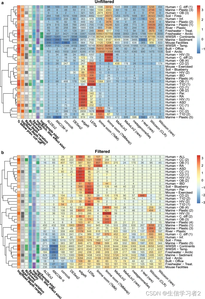
总结
该研究证实,上述不同差异分析方法识别出了截然不同的数量和显著ASV(扩增序列变体)集合,结果依赖于数据预处理。对于许多方法来说,识别出的特征数量与数据的某些方面相关,如样本大小、测序深度以及群落差异的效应大小。ALDEx2和ANCOM-II在不同研究中产生最一致的结果,并且与不同方法结果交集的一致性最好。