1. 概述

根据所拥有的数据，可以使用三种不同的机器学习方法，包括监督学习、半监督学习和无监督学习。

在监督学习中，根据已标记数据，因此可以确定输出是关于输入的正确值。通过半监督学习，用户将拥有一个大型数据集，其中一些数据已标记，但大部分未标记。由于涵盖了大量真实世界的数据，针对性标记每个数据点的成本可能很高，这就可以通过结合使用监督学习和非监督学习来解决这个问题。

无监督学习意味着我们拥有一个完全未标记的数据集，用户不知道数据中是否隐藏了任何模式，所以需将其留给算法去寻找它能找到的任何东西。这正是聚类算法的用武之地，它针对的是无监督学习问题。

聚类是一项无监督的机器学习任务，有时亦将其称为聚类分析。使用聚类算法意味着将为算法提供大量没有标签的输入数据，并让它在数据中找到它可以找到的任何分组。这些分组称为簇，簇是一组数据点，这些数据点基于它们与周围数据点的关系而彼此相似。聚类用于特征工程或模式发现之类的场景。

当我们从一无所知的数据入手时，聚类获得分组可能是对数据获得一些洞察或初探数据内部结构的好方法。

2.聚类方法

有不同类型的聚类算法可以处理具有各种特性的数据。通常可将聚类算法分为基于密度、基于分布、基于质心、基于层次等类别。

2.1基于密度（Density-based）

在基于密度的聚类中，数据按数据点密度低的区域包围数据点密度高的区域进行分组。基本上，该算法会找到数据点密集的地方并形成我们常说的“簇”。

簇可以是任何形状，不受预期条件的限制。这种类型的聚类算法不会尝试将异常值分配给簇，因此聚类后它们会被作为噪声点予以忽略或剔除。

2.2基于分布（Distribution-based）

使用基于分布的聚类方法，所有数据点都被视为基于它们属于给定簇的概率分布的一部分。

它是这样工作的：有一个中心点，随着数据点与中心的距离增加，它成为该簇一部分的概率会降低。

如果我们不确定数据的分布情况，我们应该考虑使用不同类型的算法。

2.3基于质心（Centroid-based）

基于质心的聚类是我们可能听说得最多的一种。它对我们给它的初始参数有点敏感，但它又快又高效。

这些类型的算法根据数据中的多个质心来分离数据点。每个数据点根据其与质心的平方距离分配给一个簇。这是最常用的聚类类型。

2.4基于层次（Hierarchical-based）

基于层次的聚类通常用于层次数据，就像我们从公司数据库或分类法中获得的那样。它构建了一个簇树，因此所有内容都是自上而下组织的。这比其他聚类类型更具限制性，但它非常适合特定类型的数据集。

3.聚类的应用场景

当我们有一组未标记的数据时，我们很可能会使用某种无监督学习算法。有许多不同的无监督学习技术，例如神经网络、强化学习和聚类。我们要使用的特定算法类型将具体取决于我们的数据特征与结构。

当我们尝试进行异常检测以尝试查找数据中的异常值时，我们可能希望使用聚类。它有助于找到那些簇组并显示确定数据点是否为异常值的边界。

当不确定使用何种机器学习模型时，聚类可以用来找出数据中突出内容的模式，从而更好理解数据。

聚类对于探索我们一无所知的数据特别有用。找出哪种类型的聚类算法效果最好可能需要一些时间，但当我们这样做时，我们将获得对数据的准确见解，从中甚至可以发现我们从未想到过的某种关联。

聚类的一些实际应用包括保险中的欺诈检测、图书馆中的图书分类以及市场营销中的客户或群体细分。它还可以用于更大的问题，例如地震分析或城市规划等。

4.常用的几种聚类算法

现在我们已经了解聚类算法的工作原理和可用的不同类型的一些背景知识，我们可以讨论在实践中经常看到的各种算法。在 Python的sklearn 库中的示例数据集上实施这些算法。具体来说，使用 sklearn 库中的make_classification数据集来演示不同的聚类算法为何不适合所有聚类问题。

4.1 K-means

K-均值聚类是最常用的聚类算法。它是一种基于质心的算法，也是最简单的无监督学习算法。

该算法试图最小化簇内数据点的方差。这也是大多数人接触无监督机器学习的方式。

K-means 最适用于较小的数据集，因为它会遍历所有数据点。这意味着如果数据集中有大量数据点，则需要更多时间对数据点进行分类。

由于这是 k-means 聚类数据点的方式，因此它不能很好地扩展。具体实现见如下代码。

from numpy import unique
from numpy import where
from sklearn.datasets import make_classification
from sklearn.cluster import KMeans
from matplotlib import pyplot

# initialize the data set we'll work with
training_data, _ = make_classification(
    n_samples=1000,
    n_features=2,
    n_informative=2,
    n_redundant=0,
    n_clusters_per_class=1,
    random_state=4
)

# define the model
kmeans_model = KMeans(n_clusters=2)

kmeans_model.fit(training_data)

kmeans_result = kmeans_model.predict(training_data)

# assign each data point to a cluster
# kmeans_result = kmeans_model.fit_predict(training_data)

# get all of the unique clusters
kmeans_clusters = unique(kmeans_result)

# plot the KMeans clusters
for kmeans_cluster in kmeans_clusters:
    # get data points that fall in this cluster
    index = where(kmeans_result == kmeans_cluster)
    # make the plot
    pyplot.scatter(training_data[index, 0], training_data[index, 1])

# show the KMeans plot
pyplot.show()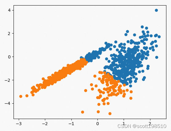

4.2 Mini Batch K-Means

Mini Batch K-Means是K-Means的一个修改版本，它使用小批量样本而不是整个数据集来更新聚类质心，这可以使其在大型数据集上更快，并且可能对统计噪声更为鲁棒。该算法的缺点是速度提升会降低聚类簇的质量。

通过提出将小批量优化用于k均值聚类。与经典的批处理算法相比，这将计算成本降低了几个数量级，同时产生了比在线随机梯度下降更好的解决效果。具体实现见如下代码。

from numpy import unique
from numpy import where
from sklearn.datasets import make_classification
from sklearn.cluster import MiniBatchKMeans
from matplotlib import pyplot
# define dataset
training_data, _ = make_classification(n_samples=1000,
                           n_features=2,
                           n_informative=2,
                           n_redundant=0,
                           n_clusters_per_class=1,
                           random_state=4)
# define the model
model = MiniBatchKMeans(n_clusters=2)
# fit the model
model.fit(training_data)
# assign a cluster to each example
kmeans_result = model.predict(training_data)
# retrieve unique clusters
clusters = unique(kmeans_result)
# create scatter plot for samples from each cluster
for cluster in clusters:
    # get row indexes for samples with this cluster
    index = where(kmeans_result == cluster)
    # create scatter of these samples
    pyplot.scatter(training_data[index, 0], training_data[index, 1])
# show the plot
pyplot.show()

4.3 DBSCAN

DBSCAN 代表具有噪声的应用程序的基于密度的空间聚类。与 k-means 不同，它是一种基于密度的聚类算法。这是在数据集中查找离群点的好算法。它根据不同区域数据点的密度发现任意形状的聚类。它按低密度区域分隔区域，以便它可以检测高密度簇之间的异常值。在处理奇形怪状的数据时，该算法优于 k-means。

DBSCAN 使用两个参数来确定聚类的定义方式：minPts（一个被认为是高密度区域需要聚类在一起的最小数据点数）和eps（用于确定一个数据点与其它属于同一个簇的数据点的距离阈值）。

选择正确的初始参数对于该算法的工作至关重要。具体实现见如下代码。

from numpy import unique
from numpy import where
from matplotlib import pyplot
from sklearn.datasets import make_classification
from sklearn.cluster import DBSCAN

# initialize the data set we'll work with
training_data, _ = make_classification(
    n_samples=1000,
    n_features=2,
    n_informative=2,
    n_redundant=0,
    n_clusters_per_class=1,
    random_state=4
)

# define the model
dbscan_model = DBSCAN(eps=0.25, min_samples=9)

# train the model
# dbscan_model.fit(training_data)

# assign each data point to a cluster
dbscan_result = dbscan_model.fit_predict(training_data)

# get all of the unique clusters
dbscan_clusters = unique(dbscan_result)

# plot the DBSCAN clusters
for dbscan_cluster in dbscan_clusters:
    # get data points that fall in this cluster
    index = where(dbscan_result == dbscan_cluster)
    # make the plot
    pyplot.scatter(training_data[index, 0], training_data[index, 1])

# show the DBSCAN plot
pyplot.show()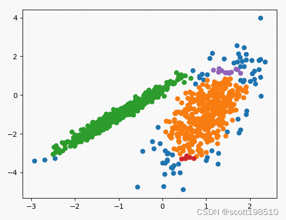

4.4 Gaussian-Mixture Model

k-means 的问题之一是数据需要遵循某种圆形区域的范式。k-means 计算数据点之间距离的方式与圆形路径有关，因此非圆形数据无法正确聚类。这是高斯混合模型解决的问题。我们不需要圆形数据就可以正常工作。

高斯混合模型使用多个高斯分布来拟合任意形状的数据。在这个混合模型中有几个单一的高斯模型充当隐藏层。因此，该模型计算数据点属于特定高斯分布的概率，这就是它将属于的簇。具体实现如下。

from numpy import unique
from numpy import where
from matplotlib import pyplot
from sklearn.datasets import make_classification
from sklearn.mixture import GaussianMixture

# initialize the data set we'll work with
training_data, _ = make_classification(
    n_samples=1000,
    n_features=2,
    n_informative=2,
    n_redundant=0,
    n_clusters_per_class=1,
    random_state=4
)

# define the model
gaussian_model = GaussianMixture(n_components=2)

# train the model
gaussian_model.fit(training_data)

# assign each data point to a cluster
gaussian_result = gaussian_model.predict(training_data)

# get all of the unique clusters
gaussian_clusters = unique(gaussian_result)

# plot Gaussian Mixture the clusters
for gaussian_cluster in gaussian_clusters:
    # get data points that fall in this cluster
    index = where(gaussian_result == gaussian_cluster)
    # make the plot
    pyplot.scatter(training_data[index, 0], training_data[index, 1])

# show the Gaussian Mixture plot
pyplot.show()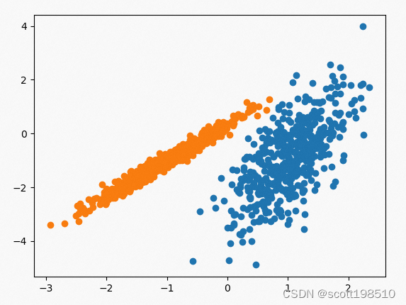

4.5 BIRCH

Balance Iterative Reducing and Clustering using Hierarchies (BIRCH) 算法在大型数据集上比 k-means 算法效果更好。它将数据分解成summaries 后再聚类，而不是基于原始数据点直接聚类。summaries 包含尽可能多的关于数据点的分布信息。

该算法通常与其他聚类算法一起使用，因为其他聚类技术可用于 BIRCH 生成的summaries 。

BIRCH 算法的主要缺点是它仅适用于数字数据值。除非进行一些必要的数据转换，否则不能将其用于分类值。具体实现见如下代码。

from numpy import unique
from numpy import where
from matplotlib import pyplot
from sklearn.datasets import make_classification
from sklearn.cluster import Birch

# initialize the data set we'll work with
training_data, _ = make_classification(
    n_samples=1000,
    n_features=2,
    n_informative=2,
    n_redundant=0,
    n_clusters_per_class=1,
    random_state=4
)

# define the model
birch_model = Birch(threshold=0.03, n_clusters=2)

# train the model
birch_model.fit(training_data)

# assign each data point to a cluster
birch_result = birch_model.predict(training_data)

# get all of the unique clusters
birch_clusters = unique(birch_result)

# plot the BIRCH clusters
for birch_cluster in birch_clusters:
    # get data points that fall in this cluster
    index = where(birch_result == birch_cluster)
    # make the plot
    pyplot.scatter(training_data[index, 0], training_data[index, 1])

# show the BIRCH plot
pyplot.show()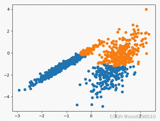

4.6 Affinity Propagation

类同传播聚类也称之为亲密度传播聚类（Affinity Propagation），这种聚类算法在聚类数据的方式上与其他算法完全不同。每个数据点都与所有其他数据点进行信息传递，让彼此知道它们有多相似，并开始揭示数据中的簇。我们不必在初始化参数中预先设定该算法期望有多少个簇。

当信息在数据点之间发送时，会找到称为样本的数据集，它们代表簇。

在数据点相互传递消息并就哪个数据点最能代表簇达成共识后，就会找到一个范例。

当我们不确定期望有多少簇时，例如在计算机视觉问题中，这是一个很好的算法。具体实现见如下代码。

from numpy import unique
from numpy import where
from matplotlib import pyplot
from sklearn.datasets import make_classification
from sklearn.cluster import AffinityPropagation

# initialize the data set we'll work with
training_data, _ = make_classification(
    n_samples=1000,
    n_features=2,
    n_informative=2,
    n_redundant=0,
    n_clusters_per_class=1,
    random_state=4
)

# define the model
model = AffinityPropagation(damping=0.7)

# train the model
model.fit(training_data)

# assign each data point to a cluster
result = model.predict(training_data)

# get all of the unique clusters
clusters = unique(result)

# plot the clusters
for cluster in clusters:
    # get data points that fall in this cluster
    index = where(result == cluster)
    # make the plot
    pyplot.scatter(training_data[index, 0], training_data[index, 1])

# show the plot
pyplot.show()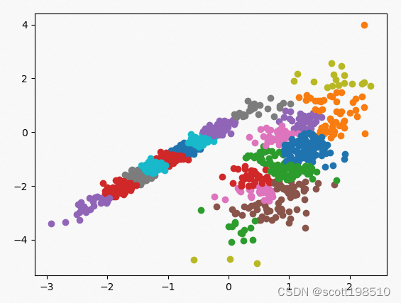

4.7 Mean-Shift

这是另一种对处理图像和计算机视觉处理特别有用的算法。

Mean-shift 类似于 BIRCH 算法，因为它也可以在没有设置初始簇数的情况下找到簇。

这是一种层次聚类算法，但缺点是在处理大型数据集时无法很好地扩展。

它通过迭代所有数据点并将它们移向pattern来工作。本文中的pattern是一个区域中数据点的高密度区域。

这就是为什么我们可能会听到将此算法称为模式搜索算法的原因。它将对每个数据点进行此迭代过程，并将它们移动到更靠近其他数据点的位置，直到所有数据点都已分配给一个簇。具体实现见如下代码。

from numpy import unique
from numpy import where
from matplotlib import pyplot
from sklearn.datasets import make_classification
from sklearn.cluster import MeanShift

# initialize the data set we'll work with
training_data, _ = make_classification(
    n_samples=1000,
    n_features=2,
    n_informative=2,
    n_redundant=0,
    n_clusters_per_class=1,
    random_state=4
)

# define the model
mean_model = MeanShift()

# assign each data point to a cluster
mean_result = mean_model.fit_predict(training_data)

# get all of the unique clusters
mean_clusters = unique(mean_result)

# plot Mean-Shift the clusters
for mean_cluster in mean_clusters:
    # get data points that fall in this cluster
    index = where(mean_result == mean_cluster)
    # make the plot
    pyplot.scatter(training_data[index, 0], training_data[index, 1])

# show the Mean-Shift plot
pyplot.show()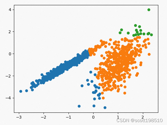

4.8 OPTICS

OPTICS 代表用于识别聚类结构的排序点。它是一种类似于 DBSCAN 的基于密度的算法，但它更好，因为它可以在密度不同的数据中找到有意义的聚类。它通过对数据点进行排序来实现这一点，以便最近的点是排序中的邻居。

这使得检测不同密度的簇变得更加容易。OPTICS 算法只对每个数据点处理一次，类似于 DBSCAN（尽管它运行速度比 DBSCAN 慢）。还为每个数据点存储了一个特殊的距离，指示该点属于特定的簇。

具体实现见如下代码。

from numpy import unique
from numpy import where
from matplotlib import pyplot
from sklearn.datasets import make_classification
from sklearn.cluster import OPTICS

# initialize the data set we'll work with
training_data, _ = make_classification(
    n_samples=1000,
    n_features=2,
    n_informative=2,
    n_redundant=0,
    n_clusters_per_class=1,
    random_state=4
)

# define the model
optics_model = OPTICS(eps=0.75, min_samples=10)

# assign each data point to a cluster
optics_result = optics_model.fit_predict(training_data)

# get all of the unique clusters
optics_clusters = unique(optics_clusters)

# plot OPTICS the clusters
for optics_cluster in optics_clusters:
    # get data points that fall in this cluster
    index = where(optics_result == optics_cluster)
    # make the plot
    pyplot.scatter(training_data[index, 0], training_data[index, 1])

# show the OPTICS plot
pyplot.show()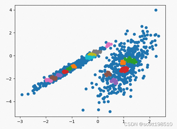

4.9 Agglomerative clustering

这是最常见的层次聚类算法。它用于根据彼此之间的相似程度将对象分组到簇中。

这也是一种自下而上的聚类方式，其中每个数据点都分配给自己的簇。然后这些簇连接在一起。

在每次迭代中，合并相似的簇，直到所有数据点都属于一个大根簇。

凝聚聚类最擅长寻找小簇。最终结果看起来像一个树状图，以便我们可以在算法完成时轻松地可视化簇。

具体实现见如下代码。

from numpy import unique
from numpy import where
from matplotlib import pyplot
from sklearn.datasets import make_classification
from sklearn.cluster import AgglomerativeClustering

# initialize the data set we'll work with
training_data, _ = make_classification(
    n_samples=1000,
    n_features=2,
    n_informative=2,
    n_redundant=0,
    n_clusters_per_class=1,
    random_state=4
)

# define the model
agglomerative_model = AgglomerativeClustering(n_clusters=2)

# assign each data point to a cluster
agglomerative_result = agglomerative_model.fit_predict(training_data)

# get all of the unique clusters
agglomerative_clusters = unique(agglomerative_result)

# plot the clusters
for agglomerative_cluster in agglomerative_clusters:
    # get data points that fall in this cluster
    index = where(agglomerative_result == agglomerative_cluster)
    # make the plot
    pyplot.scatter(training_data[index, 0], training_data[index, 1])

# show the Agglomerative Hierarchy plot
pyplot.show()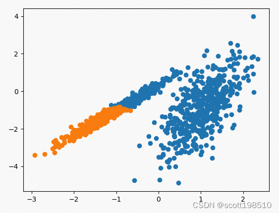

4.10 Spectral clustering

谱聚类演化于图论，此后由于其表现出优秀的性能被广泛应用于聚类分析中，对比其他无监督聚类（如kmeans），spectral clustering的优点主要有以下：

1.过程对数据结构并没有太多的假设要求，如kmeans则要求数据为凸集。
2.可以通过构造稀疏similarity graph，使得对于更大的数据集表现出明显优于其他算法的计算速度。
3.由于spectral clustering是对图切割处理，不会存在像kmesns聚类时将离散的小簇聚合在一起的情况。
4.无需像GMM一样对数据的概率分布做假设。

from numpy import unique
from numpy import where
from sklearn.datasets import make_classification
from sklearn.cluster import SpectralClustering
from matplotlib import pyplot
# define dataset
training_data, _ = make_classification(n_samples=1000,
                           n_features=2,
                           n_informative=2,
                           n_redundant=0,
                           n_clusters_per_class=1,
                           random_state=4)

# define the model
model = SpectralClustering(n_clusters=2)

# fit model and predict clusters
spectral_result = model.fit_predict(training_data)

# retrieve unique clusters
clusters = unique(spectral_result)

# create scatter plot for samples from each cluster
for cluster in clusters:
    # get row indexes for samples with this cluster
    index = where(spectral_result == cluster)
    # create scatter of these samples
    pyplot.scatter(training_data[index, 0], training_data[index, 1])
    
# show the plot
pyplot.show()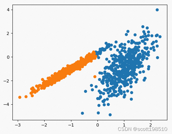

4.11 其他聚类算法

我们已经介绍了10种顶级聚类算法，但还有更多可用的算法。有一些经过专门调整的聚类算法可以快速准确地处理特定的数据。

还有另一种与Agglomerative方法相反的分层算法。它从自上而下的簇策略开始。所以它将从一个大的根簇开始，然后从那里分解出各个小簇。

这被称为Divisive Hierarchical聚类算法。有研究表明，这会创建比凝聚聚类更准确的层次结构，但它要复杂得多。

4.其他想法

需要注意的是，聚类算法需要考虑尺度问题。我们的数据集可能有数百万个数据点，并且由于聚类算法通过计算所有数据点对之间的相似性来工作，因此我们最终可能会得到一个无法很好扩展的算法，有必要对聚类的数据集进行尺度或规模上的处理。

5. 结论

聚类算法是从旧数据中学习新事物的好方法。有时使用者会对得到的结果簇感到惊讶，它可能会帮助使用者理解问题。

将聚类用于无监督学习的最酷的事情之一是可以在监督学习问题中使用聚类的结果作为标记值。

簇可能是我们在完全不同的数据集上使用的新功能！我们几乎可以对任何无监督机器学习问题使用聚类，但前提是请确保我们知道如何分析结果的准确性。