概述

• 说话人识别中的损失函数分为基于多类别分类的损失函数，和端到端的损失函数（也叫基于度量学习的损失函数），关于这些损失函数的理论部分，可参考说话人识别中的损失函数
• 本文主要关注这些损失函数的实现，此外，文章说话人识别中的损失函数中，没有详细介绍基于多类别分类的损失函数，因此本文会顺便补足这一点
• 本文持续更新

Softmax Loss

• 先看Softmax Loss，完整的叫法是Cross-entropy Loss with Softmax，主要由三部分组成

  • Fully Connected：将当前样本的嵌入码（embedding），变换成长度为类别数的向量（通常称为Logit），公式如下
    $$y=Wx+b$$
    其中

    • x是特征向量，长度为$embed\text{-}dim$
    • W是权重矩阵，维度为$[n\text{-}classes,embed\text{-}dim]$，$n\text{-}classes$为类别数
    • b是偏置向量，长度为$n\text{-}classes$
    • Logit中的每一个值，对应W的每一行与x逐项相乘再相加，然后与b中的对应项再相加

  • Softmax：将Logit变换成多类别概率分布Probability，不改变向量长度，公式如下（取 $N=n\text{-}classes-1$）
    $$y_i=\frac{e^{x_i}}{{\sum }_{i=0}^N{e}^{x_i}}$$
    

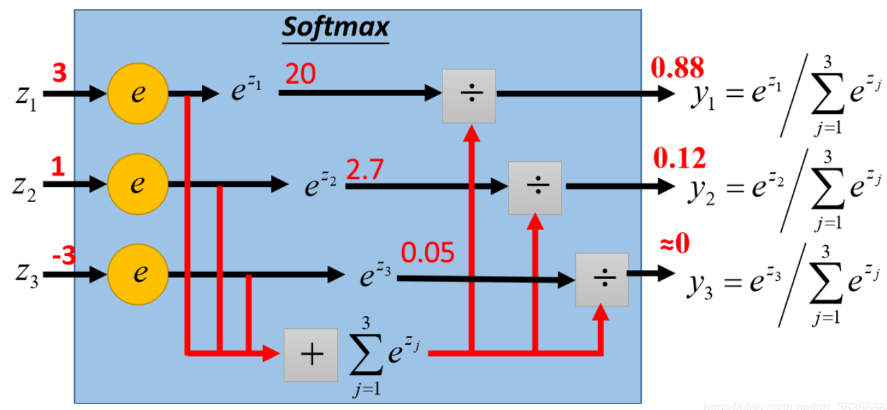
    • 本质上是max函数的软化版本，将不可导的max函数变得可导
    • 因此需要像max函数那样，具有最大值主导的特点，上图中
      $$softmax([3,1,-3])=[0.88,0.12,0]$$
    • 又因为输出是多类别概率分布，因此Probability的每一项相加等于1
      $$\sum _{i=0}^N{y}_i=1$$
    • 但是当Logit的值都比较小时，比如：$[0,1]$，最大值主导的效果不明显
      $$softmax([0.1,0.3,0.5,0.7,0.9])=[0.1289,0.1574,0.1922,0.2348,0.2868]$$

  • Cross-entropy（交叉熵）：将Ground Truth（基本事实）的One-hot Vector（记为$P$）与Probability（记为$Q$）计算相似度，输出是标量。交叉熵的值越小，Probability与One-hot Vector越相似，公式如下
    $$L_{CE}(P,Q)=-\sum _{i=0}^N{p}_i\log (q_i)$$

    • One-hot Vector的长度与Probability一致，即等于类别数$N$，形式为$[0,0,...,1,...,0]$，即GT是哪个类，哪个类对应的下标就为1
    • 设One-hot Vector值为1的下标为$j$，上式可简化为
      $$L_{Softmax}(P,Q)=-\log (q_j)=-\log (\frac{e^{x_j}}{{\sum }_{i=0}^N{e}^{x_i}})$$
• 在上述的过程中，如果用tensor.scatter_来实现One-hot Vector是比较难懂的，完整PyTorch代码如下

  import torch
  import torch.nn.functional as F
  import torch.nn as nn
  
  embed_dim = 5
  num_class = 10
  device = torch.device("cuda" if torch.cuda.is_available() else "cpu")
  
  x = torch.tensor([0.1, 0.3, 0.5, 0.7, 0.9])
  x.unsqueeze_(0)  # 模拟batch-size，就地在dim = 0插入维度，此时x的维度为[1,5]
  x = x.expand(2, embed_dim)  # 直接堆叠x，使batch-size = 2，此时x的维度为[2,5]
  x = x.float().to(device)
  
  # label是长度为batch-size的向量，每个值是GT的下标，维度为[2]
  label = torch.tensor([0, 5])
  label = label.long().to(device)
  
  weight = nn.Parameter(torch.FloatTensor(num_class, embed_dim)).to(device)
  nn.init.xavier_uniform_(weight)  # 初始化权重矩阵
  logit = F.linear(x, weight)  # 取消偏置向量
  
  probability = F.softmax(logit, dim=1)  # 维度为[2,10]
  
  # one_hot的数据类型与设备要和x相同，维度和Probability相同[2,10]
  one_hot = x.new_zeros(probability.size())
  # 根据label，就地得到one_hot，步骤如下
  	# scatter_函数：Tensor.scatter_(dim, index, src, reduce=None)
  	# 先把label的维度变为[2,1]，然后根据label的dim = 1(参数中的src)上的值
  	# 作为one_hot的dim = 1(参数中的dim)上的下标，并将下标对应的值设置为1
  	# 由于label的dim = 1上的值只有一个，所以是One-hot，如果label维度为[2,2]，则为Two-hot
  	# 如果label维度为[2,k]，则为K-hot
  one_hot.scatter_(1, label.view(-1, 1).long(), 1)
  # 等价于
  # one_hot = F.one_hot(label, num_class).float().to(device)
  # 但是F.one_hot只能构造One-hot，Tensor.scatter_可以构造K-hot
  
  # 对batch中每个样本计算loss，并求均值
  loss = 0
  for P, Q in zip(one_hot, probability):
      loss += torch.log((P * Q).sum())
  loss /= -one_hot.size()[0]
  # 等价于
  # loss = F.cross_entropy(logit, label)
  

• 上述PyTorch代码要看懂，是之后魔改Softmax Loss的基础

AAM-Softmax（ArcFace）

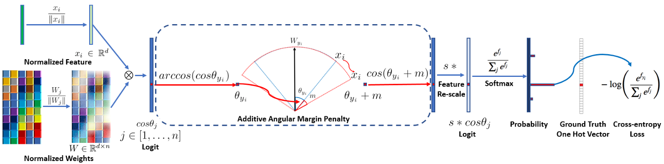
• AAM-Softmax（Additive Angular Margin Loss，也叫ArcFace）出自人脸识别，是说话人识别挑战VoxSRC近年冠军方案的基础损失函数，是基于Softmax Loss进行改进而来的。步骤如下
  

  • 取消偏置向量，根据上文，Logit中的每一个值，对应W的每一行$w_i$与x逐项相乘再相加，即$y_i=w_{i}x$

  • 把$w_i$和$x$都单位化
    $$w_i^{\prime }=\frac{w_i}{||w_i||},x^{\prime }=\frac{x}{||x||}$$

  • 计算Logit，此时Logit中的每一个值如下，即$w_i$和$x$的夹角的余弦值，记为${\theta }_i$
    $$y_i=w_i^{\prime }{x}^{\prime }=\frac{w_i}{||w_i||}\frac{x}{||x||}=\cos <w_i,x>=\cos {\theta }_i$$

  • 权重矩阵W的每一行，本质上是神经网络学习到的每个说话人的中心向量（中心点），关于说话人的中心点，可参考说话人识别中的损失函数中的端到端损失函数。端到端的损失函数，直接利用每个batch中属于不同说话人的样本，计算对应说话人的中心点；而基于多类别分类的损失函数，则是通过学习，得到每个说话人的中心点

  • 因此，将$w_i$和$x$单位化后，再计算Softmax Loss，可以视作是对当前样本嵌入码与每一个说话人中心点，计算余弦相似度向量，对余弦相似度向量进行Softmax Loss优化。根据上文，当Logit的值都比较小时，比如：$[0,1]$，Softmax最大值主导的效果不明显，所以单位化后计算的Logit，需要进行伸缩（Scale），即$y_i=s\ast y_i=s\cos {\theta }_i$。此时再计算Softmax Loss，如下
    $$L=-\log (\frac{e^{s\cos {\theta }_j}}{{\sum }_{i=0}^N{e}^{s\cos {\theta }_i}})$$

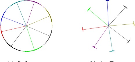
  • 用此时的Softmax Loss，训练2维嵌入码，然后取8个类，对这8个类的大量样本，计算嵌入码，绘制到图上，如下面左图所示。发现这8个类类间是可分的，但是类内却没有聚合，我们希望这8个类能够像下面右图那样，不仅类间可分，而且类内聚合
    

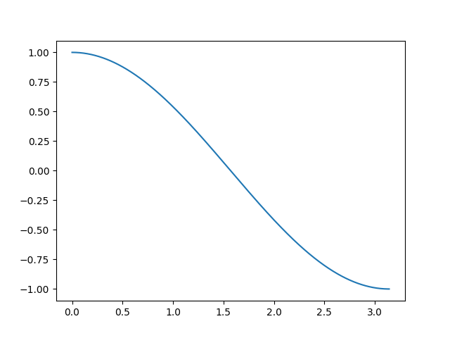
  • 首先要明确：两个向量的夹角范围为$[0,\pi ]$，夹角余弦值范围为$[-1,1]$，并且单调递减，如下图所示
    

  • 训练时，对嵌入码和GT说话人中心点的夹角，施加额外的惩罚，惩罚后，该夹角变大，从而余弦值变小，神经网络需要将余弦值重新变大，才能使该嵌入码正确分类。测试时，用嵌入码与不同的嵌入码直接计算相似度，此时没有惩罚，从而实现类间可分和类内聚合

  • AAM-Softmax中，直接将GT夹角加上一个值$m$（通常称为margin），从而Logit中GT对应的值变为$y_j=s\cos ({\theta }_j+m)$，Logit中其他的值不变，仍为$s\cos {\theta }_i$。此时再计算Softmax Loss，如下
    $$L=-\log (\frac{e^{s\cos ({\theta }_j+m)}}{e^{s\cos ({\theta }_j+m)}+{\sum }_{i=0,i\ne j}^N{e}^{s\cos {\theta }_i}})$$

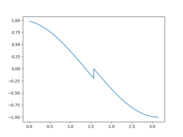
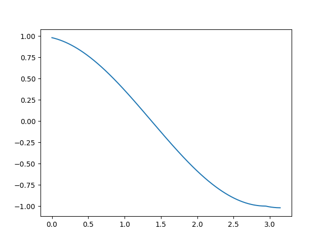
• 在上述的过程中，施加额外的惩罚这一步，有不同的情况需要讨论，先看forward函数

  def forward(self, input, label):
  	# input即上述的x，label与上述要求一致
  	# 计算cos(theta)，F.normalize默认对dim = 1施加l2-norm
  	cosine = F.linear(F.normalize(input), F.normalize(self.weight))
  	
  	# 计算sin(theta)
  	sine = torch.sqrt(1.0 - torch.pow(cosine, 2))
  	
  	# cos(theta + m) = cos(theta)cos(m) - sin(theta)sin(m)
  	phi = cosine * self.cos_m - sine * self.sin_m
  	
  	# easy_margin表示只将cos(theta) > 0的余弦值惩罚为cos(theta + m)
  	# cos(theta) <= 0的余弦值仍为cos(theta)
  	# 惩罚后的余弦值，范围为[-1, cos(m)]
  	if self.easy_margin:
  	  phi = torch.where(cosine > 0, phi, cosine)
  	
  	# 否则，对全区间施加惩罚，但不都是惩罚为(theta + m)
  	# 取th = -cos(m)
  	# 将cos(theta) > th的余弦值惩罚为(theta + m)
  	# 将cos(theta) <= th的余弦值惩罚为cos(theta) + cos(m) - 1
  	# 惩罚后的余弦值，范围为[cos(m) - 2, cos(m)]
  	else:
  	  ########
  	  # 主流代码会将cos(theta) <= th的余弦值
  	  # 惩罚为m*sin(m)，难以理解，在此不采用
  	  # phi = torch.where(cosine > self.th, phi, cosine - self.mm)
  	  phi = torch.where(cosine > self.th, phi, cosine - self.mmm)
  	  ########
  	
  	# 构造One-hot Vector
  	one_hot = input.new_zeros(cosine.size())
  	one_hot.scatter_(1, label.view(-1, 1).long(), 1)
  	
  	# 只有GT对应的余弦值被惩罚，其他余弦值仍为cos(theta)
  	output = (one_hot * phi) + ((1.0 - one_hot) * cosine)
  	
  	# 伸缩
  	output *= self.scale
  	
  	# 返回的是logit
  	return output
  

• 如果采用easy-margin，会导致GT余弦值较大的不连续
  

• 不采用easy-margin，GT余弦值能变得连续
  

• 最后是AAM-Softmax的完整PyTorch代码

  class ArcMarginProduct(nn.Module):
      r"""Implement of large margin arc distance: :
          Args:
              in_features: size of each input sample
              out_features: size of each output sample
              scale: norm of input feature
              margin: margin
              cos(theta + margin)
          """
  
      def __init__(self,
                   in_features,
                   out_features,
                   scale=32.0,
                   margin=0.2,
                   easy_margin=False):
          super(ArcMarginProduct, self).__init__()
          self.in_features = in_features
          self.out_features = out_features
          self.scale = scale
          self.margin = margin
          self.weight = nn.Parameter(torch.FloatTensor(out_features,
                                                       in_features))
          nn.init.xavier_uniform_(self.weight)
  
          self.easy_margin = easy_margin
          self.cos_m = math.cos(margin)
          self.sin_m = math.sin(margin)
          self.th = math.cos(math.pi - margin)
          self.mm = math.sin(math.pi - margin) * margin
          self.mmm = 1.0 + math.cos(
              math.pi - margin)  # this can make the output more continuous
          ########
          self.m = self.margin
          ########
  	
  	# update函数可用于margin调度，类似学习率调度，只不过margin是越调度越大
      def update(self, margin=0.2):
          self.margin = margin
          self.cos_m = math.cos(margin)
          self.sin_m = math.sin(margin)
          self.th = math.cos(math.pi - margin)
          self.mm = math.sin(math.pi - margin) * margin
          self.m = self.margin
          self.mmm = 1.0 + math.cos(math.pi - margin)
          # self.weight = self.weight
          # self.scale = self.scale
  
      def forward(self, input, label):
          cosine = F.linear(F.normalize(input), F.normalize(self.weight))
          sine = torch.sqrt(1.0 - torch.pow(cosine, 2))
          phi = cosine * self.cos_m - sine * self.sin_m
          if self.easy_margin:
              phi = torch.where(cosine > 0, phi, cosine)
          else:
              ########
              # phi = torch.where(cosine > self.th, phi, cosine - self.mm)
              phi = torch.where(cosine > self.th, phi, cosine - self.mmm)
              ########
  
          one_hot = input.new_zeros(cosine.size())
          one_hot.scatter_(1, label.view(-1, 1).long(), 1)
          output = (one_hot * phi) + ((1.0 - one_hot) * cosine)
          output *= self.scale
  
          return output
  
      def extra_repr(self):
          return '''in_features={}, out_features={}, scale={},
                    margin={}, easy_margin={}'''.format(self.in_features,
                                                        self.out_features,
                                                        self.scale, self.margin,
                                                        self.easy_margin)
  

Sub-center ArcFace

• 数据集常常带有噪声，越是大的数据集，噪声越是多，常见的噪声有离群点（Outlier）噪声和标签翻转（Label-flip）噪声，关于数据噪声，可参考说话人识别的数据需求中“数据的正确性”这一节
• 大数据集的噪声清除是非常困难且昂贵的，神经网络需要能够在带有噪声（CASIA Face中噪声约有9.3%-13.0%）的数据集中，甚至是强噪声（MS1MV0中噪声约有47.1%-54.4%）的数据集中，进行训练
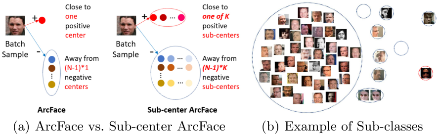
• Sub-center ArcFace就是用于在带有噪声的大规模数据集训练中，要求类内聚合和类间可分（即严格性Strictness），同时不被数据集中的噪声过度影响（即鲁棒性Robustness），的损失函数，步骤如下

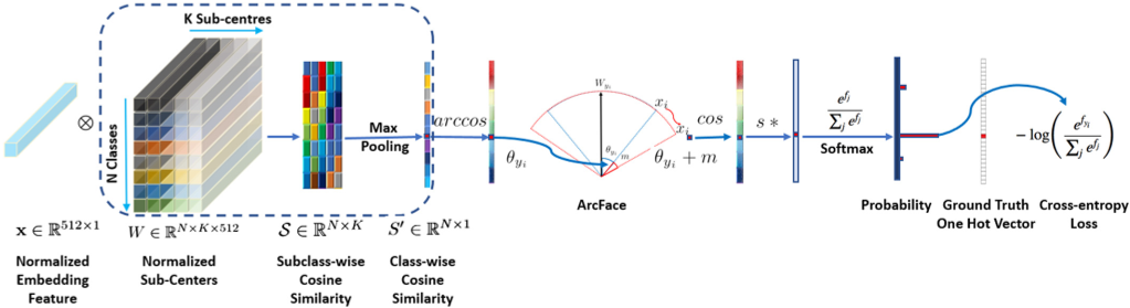
  • 根据上文，权重矩阵W的每一行，本质上是神经网络学习到的每个说话人的中心点，但是在带有噪声的数据集中， 这个学习到的中心点，可能不是非常准确

  • 可以让神经网络学习每个说话人的$K$个中心点，其中一个是正常样本（Easy clean）的中心点，称为主导中心点（Dominant Sub-center），其余是噪声（Hard or Noise）样本的中心点，称为非主导中心点（Non-dominant Sub-center）。如下图(b)所示，取$K=10$，则一共有10个圆圈，最大圆圈为主导中心点，其余圆圈为非主导中心点
    

  • 由此，W的维度从$[n\text{-}classes,embed\text{-}dim]$变成了$[n\text{-}classes,embed\text{-}dim,K]$，将嵌入码和W的每个中心点，计算余弦相似度，会得到维度为$[n\text{-}classes,K]$的相似度矩阵

  • 对相似度矩阵的每一行进行池化，会得到长为$n\text{-}classes$的向量，可以作为Logit，后续的步骤与ArcFace一致。Sub-center ArcFace的额外处理，集中在下图的蓝色虚线内
    

  • 上述对相似度矩阵的池化操作，就是平衡损失函数的Strictness和Robustness的关键。我们知道，ArcFace是对Logit中嵌入码和GT中心点的夹角，加上margin，再取cos得到GT相似度，最后对Logit计算Softmax Loss

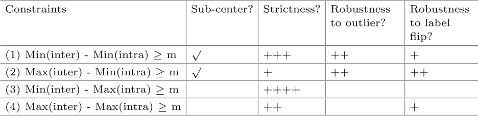
  • 因此，要分析margin与池化的协同作用，需要先把相似度矩阵映射成夹角矩阵，再作分析，如下图所示
    

  • 其中

    • $\min (inter)$表示对当前非GT的$(N-1)\ast K$个夹角进行最小值池化
    • $\max (inter)$表示对当前非GT的$(N-1)\ast K$个夹角进行最大值池化
    • $\min (intra)$表示对当前GT的$K$个夹角进行最小值池化
    • $\max (intra)$表示对当前GT的$K$个夹角进行最大值池化
    • (1) 表示，取嵌入码与距离最近的GT夹角，加上margin，再取cos得到GT相似度；取嵌入码与距离最近的非GT夹角，再取cos得到非GT相似度。此时对类内聚合的Strictness降低，从而对离群点噪声的Robustness提高；对类间可分的Strictness提高，从而对标签翻转噪声的Robustness一般
    • (2) 表示，取嵌入码与距离最近的GT夹角，加上margin，再取cos得到GT相似度；取嵌入码与距离最远的非GT夹角，再取cos得到非GT相似度。此时对类内聚合的Strictness降低，从而对离群点噪声的Robustness提高；对类间可分的Strictness降低，从而对标签翻转噪声的Robustness提高。但此时训练无法收敛，因为监督信息不够强，梯度方向不明确
    • (3) 表示，取嵌入码与距离最远的GT夹角，加上margin，再取cos得到GT相似度；取嵌入码与距离最近的非GT夹角，再取cos得到非GT相似度。此时对类内聚合的Strictness提高，从而无法学习出多个Sub-center，导致对噪声Robustness弱；对类间可分的Strictness提高。此时效果类似原始ArcFace
    • (4) 表示，取嵌入码与距离最远的GT夹角，加上margin，再取cos得到GT相似度；取嵌入码与距离最远的非GT夹角，再取cos得到非GT相似度。此时对类内聚合的Strictness提高，从而无法学习出多个Sub-center，导致对噪声Robustness弱；对类间可分的Strictness降低

  • 综上，(1) 是较优的做法，但是较大的$K$（如$K=10$），会破坏类内聚合，因为正常样本中，许多困难样本被用于学习非主导中心点，因此常取$K=3$。为增强类内聚合，还可以在神经网络判别能力较强时，去除非主导中心点，只保留主导中心点，即$K=1$，同时去除与GT主导中心点夹角小于75度的样本（这些样本可视为噪声），再用剩下的样本进行训练

• 如何检验Sub-center ArcFace的效果呢？我们希望的效果是：简单和困难样本越靠近主导中心点越好，噪声样本越靠近非主导中心点越好。因此，要检验Sub-center ArcFace的效果，可以先用强噪声的大规模数据集训练Sub-center ArcFace，之后统计训练集中，更靠近主导中心点，与更靠近非主导中心点的样本，最后检查这些样本中，哪些是正常样本，哪些是噪声样本。如下图所示
  
• 从上图中可见，相比ArcFace（图c），Sub-center ArcFace靠近主导中心点（图a）的噪声样本从38%降低到12%，不过也有4%左右的正常样本，更靠近非主导中心点（图b）
• 绝大多数的靠近主导中心点的噪声样本，夹角都大于75度，这也是上述Sub-center ArcFace最后一个步骤中的增强类内聚合，按照75度来去除噪声样本的依据。采用增强类内聚合方法后，效果如图(d)所示
• 有了ArcFace的基础，Sub-center ArcFace的PyTorch实现就比较好理解了，下面是完整代码

  class ArcMarginProduct_subcenter(nn.Module):
      r"""Implement of large margin arc distance with subcenter:
          Reference:
              Sub-center ArcFace: Boosting Face Recognition by
              Large-Scale Noisy Web Faces.
              https://ibug.doc.ic.ac.uk/media/uploads/documents/eccv_1445.pdf
          Args:
              in_features: size of each input sample
              out_features: size of each output sample
              scale: norm of input feature
              margin: margin
              cos(theta + margin)
              K: number of sub-centers
          """
  
      def __init__(self,
                   in_features,
                   out_features,
                   scale=32.0,
                   margin=0.2,
                   easy_margin=False,
                   K=3):
          super(ArcMarginProduct_subcenter, self).__init__()
          self.in_features = in_features
          self.out_features = out_features
          self.scale = scale
          self.margin = margin
  
          # subcenter
          self.K = K
  
          # initial classifier
          self.weight = nn.Parameter(
              torch.FloatTensor(self.K * out_features, in_features))
          nn.init.xavier_uniform_(self.weight)
  
          self.easy_margin = easy_margin
          self.cos_m = math.cos(margin)
          self.sin_m = math.sin(margin)
          self.th = math.cos(math.pi - margin)
          self.mm = math.sin(math.pi - margin) * margin
          self.mmm = 1.0 + math.cos(
              math.pi - margin)  # this can make the output more continuous
          ########
          self.m = self.margin
          ########
  
      def update(self, margin=0.2):
          self.margin = margin
          self.cos_m = math.cos(margin)
          self.sin_m = math.sin(margin)
          self.th = math.cos(math.pi - margin)
          self.mm = math.sin(math.pi - margin) * margin
          self.m = self.margin
          self.mmm = 1.0 + math.cos(math.pi - margin)
  
      def forward(self, input, label):
      	# 对cos(theta)的额外处理是与原始ArcFace的唯一区别
          cosine = F.linear(F.normalize(input),
                            F.normalize(self.weight))  # (batch, out_dim * k)
          cosine = torch.reshape(
              cosine, (-1, self.out_features, self.K))  # (batch, out_dim, k)
          # 取max是因为cos(theta)是相似度，与theta刚好成反比
          # 如果现在处理的是theta，则应取min，然后取cos
          cosine, _ = torch.max(cosine, 2)  # (batch, out_dim)
  
          sine = torch.sqrt(1.0 - torch.pow(cosine, 2))
          phi = cosine * self.cos_m - sine * self.sin_m
  
          if self.easy_margin:
              phi = torch.where(cosine > 0, phi, cosine)
          else:
              ########
              # phi = torch.where(cosine > self.th, phi, cosine - self.mm)
              phi = torch.where(cosine > self.th, phi, cosine - self.mmm)
              ########
  
          one_hot = input.new_zeros(cosine.size())
          one_hot.scatter_(1, label.view(-1, 1).long(), 1)
  
          output = (one_hot * phi) + ((1.0 - one_hot) * cosine)
          output *= self.scale
          
          return output
  
  	def extra_repr(self):
  		return 'in_features={}, out_features={}, scale={}, margin={}, ' \
  		       'easy_margin={}, K={}'.format(
  		          self.in_features, self.out_features, self.scale, self.margin,
  		          self.easy_margin, self.K)
  

Sub-center ArcFace/CosFace with Inter-topK

• CosFace（AM-Softmax）和ArcFace比较类似，是对嵌入码和GT中心点的余弦值，减去margin，即
  $$L=-\log (\frac{e^{s(\cos ({\theta }_j)-m)}}{e^{s(\cos ({\theta }_j)-m)}+{\sum }_{i=0,i\ne j}^N{e}^{s\cos ({\theta }_i)}})$$
• 这一过程也可以视作是：对嵌入码和非GT中心点的余弦值，加上margin，即
  $$L=-\log (\frac{e^{s\cos ({\theta }_j)}}{e^{s\cos ({\theta }_j)}+{\sum }_{i=0,i\ne j}^N{e}^{s(\cos ({\theta }_i)+m)}})$$
• 上述做法，对非GT中心点一视同仁地加上margin，这样做是次优的，因为对于一个说话人而言，有很多和TA相似的说话人，这些说话人应该被着重关注，也就是加上更大的margin，类似的想法也出现在说话人识别中的分数规范化（Score Normalization）中的AS-norm（Adaptive score Normalization）
• 具体而言，我们在嵌入码和非GT中心点的余弦值中，取前K个最大（$\text{topK}$）的余弦值，然后加上margin，记为$mp$，再对嵌入码和GT中心点的余弦值，减去margin，记为$m$，即
  $$\begin{array}{rl}L& =-\log (\frac{e^{s(\cos ({\theta }_j)-m)}}{e^{s(\cos ({\theta }_j)-m)}+{\sum }_{i=0,i\ne j}^N{e}^{s\cdot \varphi ({\theta }_i)}})\\ \varphi ({\theta }_i)& =\{\begin{array}{rl}& cos({\theta }_i)+mp,{\theta }_i\in \arg \text{topK}(cos({\theta }_i))\\ & cos({\theta }_i),Others\end{array}\end{array}$$
• 上面的式子就是CosFace with Inter-topK，同理，对于ArcFace with Inter-topK，式子为
  $$\begin{array}{rl}L& =-\log (\frac{e^{s\cos ({\theta }_j+m)}}{e^{s\cos ({\theta }_j+m)}+{\sum }_{i=0,i\ne j}^N{e}^{s\cdot \varphi ({\theta }_i)}})\\ \varphi ({\theta }_i)& =\{\begin{array}{rl}& cos({\theta }_i-mp),{\theta }_i\in \arg \text{topK}(cos({\theta }_i))\\ & cos({\theta }_i),Others\end{array}\end{array}$$
• 此外，由于上述的Sub-center和Inter-topK是相互独立的，所以可以将两者结合起来。Sub-center有助于在噪声数据集上进行训练，而Inter-topK则强调对困难样本的类间可分，当然也利于类内聚合，Sub-center ArcFace with Inter-topK的forward函数如下

  def forward(self, input, label):
  	# Sub-center ArcFace对cos(theta)的额外处理
  	cosine = F.linear(F.normalize(input),
  	                  F.normalize(self.weight))  # (batch, out_dim * k)
  	cosine = torch.reshape(
  	    cosine, (-1, self.out_features, self.K))  # (batch, out_dim, k)
  	cosine, _ = torch.max(cosine, 2)  # (batch, out_dim)
  	
  	sine = torch.sqrt(1.0 - torch.pow(cosine, 2))
  	# cos(theta + m) = cos(theta)cos(m) - sin(theta)sin(m)
  	phi = cosine * self.cos_m - sine * self.sin_m
  	# cos(theta - mp) = cos(theta)cos(mp) + sin(theta)sin(mp)
  	phi_mp = cosine * self.cos_mp + sine * self.sin_mp
  	
  	if self.easy_margin:
  	    phi = torch.where(cosine > 0, phi, cosine)
  	else:
  	    ########
  	    # phi = torch.where(cosine > self.th, phi, cosine - self.mm)
  	    phi = torch.where(cosine > self.th, phi, cosine - self.mmm)
  	    ########
  	
  	one_hot = input.new_zeros(cosine.size())
  	one_hot.scatter_(1, label.view(-1, 1).long(), 1)
  	
  	# 当需要topK时
  	if self.k_top > 0:
  	    # 先让GT余弦值减去2，从而在top_k_index中排除GT
  	    _, top_k_index = torch.topk(cosine - 2 * one_hot,
  	                                self.k_top)
          # 此时top_k_index的维度为[bs,k_top]
          # top_k_one_hot的维度与cosine相同[bs,n_classes]
          # 使用scatter_函数，可就地得到K-hot Vector，详情可参考上述Softmax Loss的代码解读
  	    top_k_one_hot = input.new_zeros(cosine.size()).scatter_(
  	        1, top_k_index, 1)
  	
  	    # 构造Logit
  	    output = (one_hot * phi) + (top_k_one_hot * phi_mp) + (
  	        (1.0 - one_hot - top_k_one_hot) * cosine)
  	# 当不需要topK时，退化为Sub-center ArcFace
  	else:
  	    output = (one_hot * phi) + ((1.0 - one_hot) * cosine)
  	
  	output *= self.scale
  	
  	return output
  

• 在实际的训练中，如果采用了margin调度，那么$m$和$mp$都需要调度。此外，如果采用大间隔微调（Large Margin Fine-tuning，利用在margin=0.2下训练好的参数，再在margin=0.5下进行微调），需要取消$mp$，完整代码如下

  class ArcMarginProduct_intertopk_subcenter(nn.Module):
      r"""Implement of large margin arc distance with intertopk and subcenter:
          Reference:
              MULTI-QUERY MULTI-HEAD ATTENTION POOLING AND INTER-TOPK PENALTY
              FOR SPEAKER VERIFICATION.
              https://arxiv.org/pdf/2110.05042.pdf
              Sub-center ArcFace: Boosting Face Recognition by
              Large-Scale Noisy Web Faces.
              https://ibug.doc.ic.ac.uk/media/uploads/documents/eccv_1445.pdf
          Args:
              in_features: size of each input sample
              out_features: size of each output sample
              scale: norm of input feature
              margin: margin
              cos(theta + margin)
              K: number of sub-centers
              k_top: number of hard samples
              mp: margin penalty of hard samples
              do_lm: whether do large margin finetune
          """
  
      def __init__(self,
                   in_features,
                   out_features,
                   scale=32.0,
                   margin=0.2,
                   easy_margin=False,
                   K=3,
                   mp=0.06,
                   k_top=5,
                   do_lm=False):
          super(ArcMarginProduct_intertopk_subcenter, self).__init__()
          self.in_features = in_features
          self.out_features = out_features
          self.scale = scale
          self.margin = margin
          self.do_lm = do_lm
  
          # intertopk + subcenter
          self.K = K
          if do_lm:  # if do LMF, remove hard sample penalty
              self.mp = 0.0
              self.k_top = 0
          else:
              self.mp = mp
              self.k_top = k_top
  
          # initial classifier
          self.weight = nn.Parameter(
              torch.FloatTensor(self.K * out_features, in_features))
          nn.init.xavier_uniform_(self.weight)
  
          self.easy_margin = easy_margin
          self.cos_m = math.cos(margin)
          self.sin_m = math.sin(margin)
          self.th = math.cos(math.pi - margin)
          self.mm = math.sin(math.pi - margin) * margin
          self.mmm = 1.0 + math.cos(
              math.pi - margin)  # this can make the output more continuous
          ########
          self.m = self.margin
          ########
          self.cos_mp = math.cos(0.0)
          self.sin_mp = math.sin(0.0)
  
      def update(self, margin=0.2):
          self.margin = margin
          self.cos_m = math.cos(margin)
          self.sin_m = math.sin(margin)
          self.th = math.cos(math.pi - margin)
          self.mm = math.sin(math.pi - margin) * margin
          self.m = self.margin
          self.mmm = 1.0 + math.cos(math.pi - margin)
  
          # hard sample margin is increasing as margin
          if margin > 0.001:
              mp = self.mp * (margin / 0.2)
          else:
              mp = 0.0
          self.cos_mp = math.cos(mp)
          self.sin_mp = math.sin(mp)
  
      def forward(self, input, label):
          cosine = F.linear(F.normalize(input),
                            F.normalize(self.weight))  # (batch, out_dim * k)
          cosine = torch.reshape(
              cosine, (-1, self.out_features, self.K))  # (batch, out_dim, k)
          cosine, _ = torch.max(cosine, 2)  # (batch, out_dim)
  
          sine = torch.sqrt(1.0 - torch.pow(cosine, 2))
          phi = cosine * self.cos_m - sine * self.sin_m
          phi_mp = cosine * self.cos_mp + sine * self.sin_mp
  
          if self.easy_margin:
              phi = torch.where(cosine > 0, phi, cosine)
          else:
              ########
              # phi = torch.where(cosine > self.th, phi, cosine - self.mm)
              phi = torch.where(cosine > self.th, phi, cosine - self.mmm)
              ########
  
          one_hot = input.new_zeros(cosine.size())
          one_hot.scatter_(1, label.view(-1, 1).long(), 1)
  
          if self.k_top > 0:
              # topk (j != y_i)
              _, top_k_index = torch.topk(cosine - 2 * one_hot,
                                          self.k_top)  # exclude j = y_i
              top_k_one_hot = input.new_zeros(cosine.size()).scatter_(
                  1, top_k_index, 1)
  
              # sum
              output = (one_hot * phi) + (top_k_one_hot * phi_mp) + (
                  (1.0 - one_hot - top_k_one_hot) * cosine)
          else:
              output = (one_hot * phi) + ((1.0 - one_hot) * cosine)
          output *= self.scale
          return output
  
      def extra_repr(self):
          return 'in_features={}, out_features={}, scale={}, margin={}, ' \
              'easy_margin={}, K={}, mp={}, k_top={}, do_lm={}'.format(
                  self.in_features, self.out_features, self.scale, self.margin,
                  self.easy_margin, self.K, self.mp, self.k_top, self.do_lm)