目录
简介
设置
下载 MosMedData:胸部CT扫描与COVID-19相关发现
加载数据和预处理
建立训练和验证数据集
数据增强
定义 3D 卷积神经网络
训练模型
模型性能可视化
通过一次 CT 扫描进行预测
政安晨的个人主页:政安晨
欢迎 👍点赞✍评论⭐收藏
收录专栏: TensorFlow与Keras机器学习实战
希望政安晨的博客能够对您有所裨益,如有不足之处,欢迎在评论区提出指正!
本文目标:训练三维卷积神经网络,预测是否存在肺炎。
简介
本示例将展示构建三维卷积神经网络(CNN)所需的步骤,以预测计算机断层扫描(CT)中是否存在病毒性肺炎。二维卷积神经网络通常用于处理 RGB 图像(3 个通道)。
三维卷积神经网络与三维卷积神经网络完全相同:它的输入是三维体积或二维帧序列(如 CT 扫描中的切片),三维卷积神经网络是学习体积数据表示的强大模型。
设置
import os
import zipfile
import numpy as np
import tensorflow as tf  # for data preprocessing

import keras
from keras import layers
下载 MosMedData:胸部CT扫描与COVID-19相关发现
在本示例中,我们使用了 MosMedData.Net 的一个子集:与 COVID-19 相关结果的胸部 CT 扫描。该数据集包括有 COVID-19 相关结果的肺部 CT 扫描,以及没有此类结果的肺部 CT 扫描。
我们将使用 CT 扫描的相关放射学结果作为标签来构建分类器,以预测是否存在病毒性肺炎。
因此,这项任务是一个二元分类问题。
# Download url of normal CT scans.
url = "https://github.com/hasibzunair/3D-image-classification-tutorial/releases/download/v0.2/CT-0.zip"
filename = os.path.join(os.getcwd(), "CT-0.zip")
keras.utils.get_file(filename, url)

# Download url of abnormal CT scans.
url = "https://github.com/hasibzunair/3D-image-classification-tutorial/releases/download/v0.2/CT-23.zip"
filename = os.path.join(os.getcwd(), "CT-23.zip")
keras.utils.get_file(filename, url)

# Make a directory to store the data.
os.makedirs("MosMedData")

# Unzip data in the newly created directory.
with zipfile.ZipFile("CT-0.zip", "r") as z_fp:
    z_fp.extractall("./MosMedData/")

with zipfile.ZipFile("CT-23.zip", "r") as z_fp:
    z_fp.extractall("./MosMedData/")
演绎展示:
Downloading data from https://github.com/hasibzunair/3D-image-classification-tutorial/releases/download/v0.2/CT-0.zip

1045162547/1045162547 ━━━━━━━━━━━━━━━━━━━━ 4s 0us/step
加载数据和预处理
文件以 Nifti 格式提供,扩展名为 .nii。为了读取扫描结果,我们使用了 nibabel 软件包。
您可以通过 pip install nibabel 安装该软件包。
CT 扫描以 Hounsfield 单位(HU)存储原始体素强度。在本数据集中,它们的范围从-1024 到 2000 以上。高于 400 的骨骼具有不同的放射性强度,因此将其作为一个较高的界限。通常使用介于 -1000 和 400 之间的阈值对 CT 扫描进行归一化处理。
为了处理数据,我们采取了以下措施:
× 我们首先将体积旋转 90 度,使方向固定下来
× 将 HU 值缩放至 0 和 1 之间。
× 调整宽度、高度和深度。
在此,我们定义了几个辅助函数来处理数据。这些函数将在建立训练和验证数据集时使用。
import nibabel as nib

from scipy import ndimage


def read_nifti_file(filepath):
    """Read and load volume"""
    # Read file
    scan = nib.load(filepath)
    # Get raw data
    scan = scan.get_fdata()
    return scan


def normalize(volume):
    """Normalize the volume"""
    min = -1000
    max = 400
    volume[volume < min] = min
    volume[volume > max] = max
    volume = (volume - min) / (max - min)
    volume = volume.astype("float32")
    return volume


def resize_volume(img):
    """Resize across z-axis"""
    # Set the desired depth
    desired_depth = 64
    desired_width = 128
    desired_height = 128
    # Get current depth
    current_depth = img.shape[-1]
    current_width = img.shape[0]
    current_height = img.shape[1]
    # Compute depth factor
    depth = current_depth / desired_depth
    width = current_width / desired_width
    height = current_height / desired_height
    depth_factor = 1 / depth
    width_factor = 1 / width
    height_factor = 1 / height
    # Rotate
    img = ndimage.rotate(img, 90, reshape=False)
    # Resize across z-axis
    img = ndimage.zoom(img, (width_factor, height_factor, depth_factor), order=1)
    return img


def process_scan(path):
    """Read and resize volume"""
    # Read scan
    volume = read_nifti_file(path)
    # Normalize
    volume = normalize(volume)
    # Resize width, height and depth
    volume = resize_volume(volume)
    return volume
让我们从类目录中读取 CT 扫描的路径。
# Folder "CT-0" consist of CT scans having normal lung tissue,
# no CT-signs of viral pneumonia.
normal_scan_paths = [
    os.path.join(os.getcwd(), "MosMedData/CT-0", x)
    for x in os.listdir("MosMedData/CT-0")
]
# Folder "CT-23" consist of CT scans having several ground-glass opacifications,
# involvement of lung parenchyma.
abnormal_scan_paths = [
    os.path.join(os.getcwd(), "MosMedData/CT-23", x)
    for x in os.listdir("MosMedData/CT-23")
]

print("CT scans with normal lung tissue: " + str(len(normal_scan_paths)))
print("CT scans with abnormal lung tissue: " + str(len(abnormal_scan_paths)))
演绎展示:
CT scans with normal lung tissue: 100
CT scans with abnormal lung tissue: 100
建立训练和验证数据集
从类目录中读取扫描数据并分配标签。对扫描数据进行下采样,使其大小为 128x128x64。将原始 HU 值的范围调整为 0 至 1。最后,将数据集分成训练子集和验证子集。
# Read and process the scans.
# Each scan is resized across height, width, and depth and rescaled.
abnormal_scans = np.array([process_scan(path) for path in abnormal_scan_paths])
normal_scans = np.array([process_scan(path) for path in normal_scan_paths])

# For the CT scans having presence of viral pneumonia
# assign 1, for the normal ones assign 0.
abnormal_labels = np.array([1 for _ in range(len(abnormal_scans))])
normal_labels = np.array([0 for _ in range(len(normal_scans))])

# Split data in the ratio 70-30 for training and validation.
x_train = np.concatenate((abnormal_scans[:70], normal_scans[:70]), axis=0)
y_train = np.concatenate((abnormal_labels[:70], normal_labels[:70]), axis=0)
x_val = np.concatenate((abnormal_scans[70:], normal_scans[70:]), axis=0)
y_val = np.concatenate((abnormal_labels[70:], normal_labels[70:]), axis=0)
print(
    "Number of samples in train and validation are %d and %d."
    % (x_train.shape[0], x_val.shape[0])
)
演绎展示:
Number of samples in train and validation are 140 and 60.数据增强
在训练过程中,我们还通过随机角度旋转来增强 CT 扫描数据。由于数据存储在形状为(样本、高度、宽度、深度)的 3 级张量中,我们在轴 4 上添加了大小为 1 的维度,以便对数据进行三维卷积。因此,新的形状为(样本、高度、宽度、深度、1)。预处理和增强技术种类繁多,本示例展示了几种简单的预处理和增强技术。
import random

from scipy import ndimage


def rotate(volume):
    """Rotate the volume by a few degrees"""

    def scipy_rotate(volume):
        # define some rotation angles
        angles = [-20, -10, -5, 5, 10, 20]
        # pick angles at random
        angle = random.choice(angles)
        # rotate volume
        volume = ndimage.rotate(volume, angle, reshape=False)
        volume[volume < 0] = 0
        volume[volume > 1] = 1
        return volume

    augmented_volume = tf.numpy_function(scipy_rotate, [volume], tf.float32)
    return augmented_volume


def train_preprocessing(volume, label):
    """Process training data by rotating and adding a channel."""
    # Rotate volume
    volume = rotate(volume)
    volume = tf.expand_dims(volume, axis=3)
    return volume, label


def validation_preprocessing(volume, label):
    """Process validation data by only adding a channel."""
    volume = tf.expand_dims(volume, axis=3)
    return volume, label
在定义训练和验证数据加载器时,训练数据会通过增强函数随机旋转不同角度的体积。请注意,训练数据和验证数据都已被重新调整为 0 至 1 之间的值。
# Define data loaders.
train_loader = tf.data.Dataset.from_tensor_slices((x_train, y_train))
validation_loader = tf.data.Dataset.from_tensor_slices((x_val, y_val))

batch_size = 2
# Augment the on the fly during training.
train_dataset = (
    train_loader.shuffle(len(x_train))
    .map(train_preprocessing)
    .batch(batch_size)
    .prefetch(2)
)
# Only rescale.
validation_dataset = (
    validation_loader.shuffle(len(x_val))
    .map(validation_preprocessing)
    .batch(batch_size)
    .prefetch(2)
)
可视化增强 CT 扫描。
import matplotlib.pyplot as plt

data = train_dataset.take(1)
images, labels = list(data)[0]
images = images.numpy()
image = images[0]
print("Dimension of the CT scan is:", image.shape)
plt.imshow(np.squeeze(image[:, :, 30]), cmap="gray")
演绎展示:
Dimension of the CT scan is: (128, 128, 64, 1)

<matplotlib.image.AxesImage at 0x7fc5b9900d50>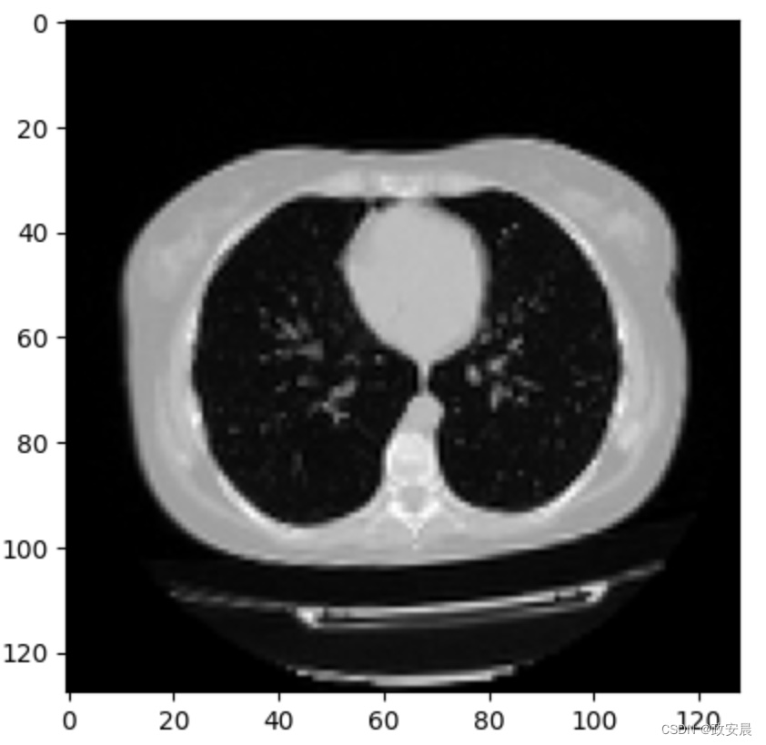
由于 CT 扫描有许多切片,因此我们可以将这些切片做成蒙太奇效果。
def plot_slices(num_rows, num_columns, width, height, data):
    """Plot a montage of 20 CT slices"""
    data = np.rot90(np.array(data))
    data = np.transpose(data)
    data = np.reshape(data, (num_rows, num_columns, width, height))
    rows_data, columns_data = data.shape[0], data.shape[1]
    heights = [slc[0].shape[0] for slc in data]
    widths = [slc.shape[1] for slc in data[0]]
    fig_width = 12.0
    fig_height = fig_width * sum(heights) / sum(widths)
    f, axarr = plt.subplots(
        rows_data,
        columns_data,
        figsize=(fig_width, fig_height),
        gridspec_kw={"height_ratios": heights},
    )
    for i in range(rows_data):
        for j in range(columns_data):
            axarr[i, j].imshow(data[i][j], cmap="gray")
            axarr[i, j].axis("off")
    plt.subplots_adjust(wspace=0, hspace=0, left=0, right=1, bottom=0, top=1)
    plt.show()


# Visualize montage of slices.
# 4 rows and 10 columns for 100 slices of the CT scan.
plot_slices(4, 10, 128, 128, image[:, :, :40])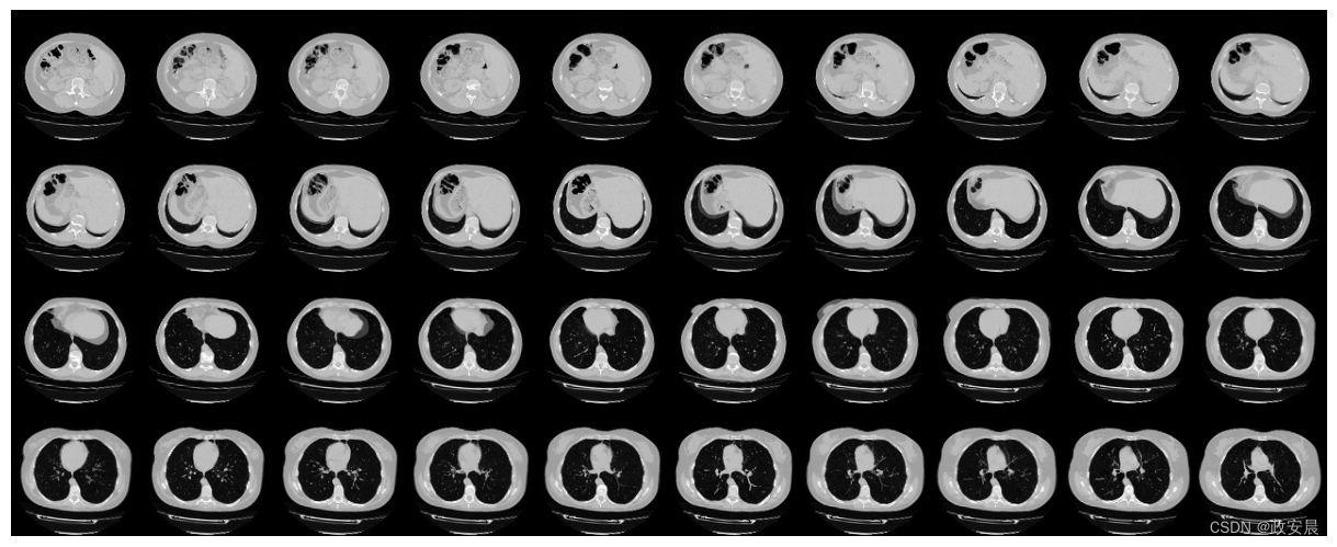
定义 3D 卷积神经网络
为使模型更易于理解,我们将其结构划分为多个区块。本示例中使用的 3D CNN 架构就是基于这篇论文。
def get_model(width=128, height=128, depth=64):
    """Build a 3D convolutional neural network model."""

    inputs = keras.Input((width, height, depth, 1))

    x = layers.Conv3D(filters=64, kernel_size=3, activation="relu")(inputs)
    x = layers.MaxPool3D(pool_size=2)(x)
    x = layers.BatchNormalization()(x)

    x = layers.Conv3D(filters=64, kernel_size=3, activation="relu")(x)
    x = layers.MaxPool3D(pool_size=2)(x)
    x = layers.BatchNormalization()(x)

    x = layers.Conv3D(filters=128, kernel_size=3, activation="relu")(x)
    x = layers.MaxPool3D(pool_size=2)(x)
    x = layers.BatchNormalization()(x)

    x = layers.Conv3D(filters=256, kernel_size=3, activation="relu")(x)
    x = layers.MaxPool3D(pool_size=2)(x)
    x = layers.BatchNormalization()(x)

    x = layers.GlobalAveragePooling3D()(x)
    x = layers.Dense(units=512, activation="relu")(x)
    x = layers.Dropout(0.3)(x)

    outputs = layers.Dense(units=1, activation="sigmoid")(x)

    # Define the model.
    model = keras.Model(inputs, outputs, name="3dcnn")
    return model


# Build model.
model = get_model(width=128, height=128, depth=64)
model.summary()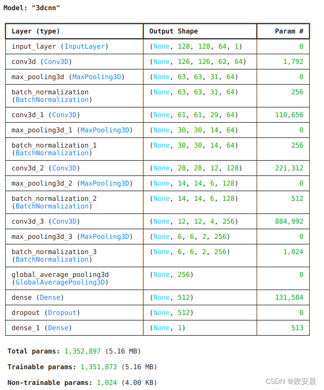
训练模型
# Compile model.
initial_learning_rate = 0.0001
lr_schedule = keras.optimizers.schedules.ExponentialDecay(
    initial_learning_rate, decay_steps=100000, decay_rate=0.96, staircase=True
)
model.compile(
    loss="binary_crossentropy",
    optimizer=keras.optimizers.Adam(learning_rate=lr_schedule),
    metrics=["acc"],
    run_eagerly=True,
)

# Define callbacks.
checkpoint_cb = keras.callbacks.ModelCheckpoint(
    "3d_image_classification.keras", save_best_only=True
)
early_stopping_cb = keras.callbacks.EarlyStopping(monitor="val_acc", patience=15)

# Train the model, doing validation at the end of each epoch
epochs = 100
model.fit(
    train_dataset,
    validation_data=validation_dataset,
    epochs=epochs,
    shuffle=True,
    verbose=2,
    callbacks=[checkpoint_cb, early_stopping_cb],
)
展示演绎:
Epoch 1/100

70/70 - 40s - 568ms/step - acc: 0.5786 - loss: 0.7128 - val_acc: 0.5000 - val_loss: 0.8744

Epoch 2/100

70/70 - 26s - 370ms/step - acc: 0.6000 - loss: 0.6760 - val_acc: 0.5000 - val_loss: 1.2741

Epoch 3/100

70/70 - 26s - 373ms/step - acc: 0.5643 - loss: 0.6768 - val_acc: 0.5000 - val_loss: 1.4767

Epoch 4/100

70/70 - 26s - 376ms/step - acc: 0.6643 - loss: 0.6671 - val_acc: 0.5000 - val_loss: 1.2609

Epoch 5/100

70/70 - 26s - 374ms/step - acc: 0.6714 - loss: 0.6274 - val_acc: 0.5667 - val_loss: 0.6470

Epoch 6/100

70/70 - 26s - 372ms/step - acc: 0.5929 - loss: 0.6492 - val_acc: 0.6667 - val_loss: 0.6022

Epoch 7/100

70/70 - 26s - 374ms/step - acc: 0.5929 - loss: 0.6601 - val_acc: 0.5667 - val_loss: 0.6788

Epoch 8/100

70/70 - 26s - 378ms/step - acc: 0.6000 - loss: 0.6559 - val_acc: 0.6667 - val_loss: 0.6090

Epoch 9/100

70/70 - 26s - 373ms/step - acc: 0.6357 - loss: 0.6423 - val_acc: 0.6000 - val_loss: 0.6535

Epoch 10/100

70/70 - 26s - 374ms/step - acc: 0.6500 - loss: 0.6127 - val_acc: 0.6500 - val_loss: 0.6204

Epoch 11/100

70/70 - 26s - 374ms/step - acc: 0.6714 - loss: 0.5994 - val_acc: 0.7000 - val_loss: 0.6218

Epoch 12/100

70/70 - 26s - 374ms/step - acc: 0.6714 - loss: 0.5980 - val_acc: 0.7167 - val_loss: 0.5069

Epoch 13/100

70/70 - 26s - 369ms/step - acc: 0.7214 - loss: 0.6003 - val_acc: 0.7833 - val_loss: 0.5182

Epoch 14/100

70/70 - 26s - 372ms/step - acc: 0.6643 - loss: 0.6076 - val_acc: 0.7167 - val_loss: 0.5613

Epoch 15/100

70/70 - 26s - 373ms/step - acc: 0.6571 - loss: 0.6359 - val_acc: 0.6167 - val_loss: 0.6184

Epoch 16/100

70/70 - 26s - 374ms/step - acc: 0.6429 - loss: 0.6053 - val_acc: 0.7167 - val_loss: 0.5258

Epoch 17/100

70/70 - 26s - 370ms/step - acc: 0.6786 - loss: 0.6119 - val_acc: 0.5667 - val_loss: 0.8481

Epoch 18/100

70/70 - 26s - 372ms/step - acc: 0.6286 - loss: 0.6298 - val_acc: 0.6667 - val_loss: 0.5709

Epoch 19/100

70/70 - 26s - 372ms/step - acc: 0.7214 - loss: 0.5979 - val_acc: 0.5833 - val_loss: 0.6730

Epoch 20/100

70/70 - 26s - 372ms/step - acc: 0.7571 - loss: 0.5224 - val_acc: 0.7167 - val_loss: 0.5710

Epoch 21/100

70/70 - 26s - 372ms/step - acc: 0.7357 - loss: 0.5606 - val_acc: 0.7167 - val_loss: 0.5444

Epoch 22/100

70/70 - 26s - 372ms/step - acc: 0.7357 - loss: 0.5334 - val_acc: 0.5667 - val_loss: 0.7919

Epoch 23/100

70/70 - 26s - 373ms/step - acc: 0.7071 - loss: 0.5337 - val_acc: 0.5167 - val_loss: 0.9527

Epoch 24/100

70/70 - 26s - 371ms/step - acc: 0.7071 - loss: 0.5635 - val_acc: 0.7167 - val_loss: 0.5333

Epoch 25/100

70/70 - 26s - 373ms/step - acc: 0.7643 - loss: 0.4787 - val_acc: 0.6333 - val_loss: 1.0172

Epoch 26/100

70/70 - 26s - 372ms/step - acc: 0.7357 - loss: 0.5535 - val_acc: 0.6500 - val_loss: 0.6926

Epoch 27/100

70/70 - 26s - 370ms/step - acc: 0.7286 - loss: 0.5608 - val_acc: 0.5000 - val_loss: 3.3032

Epoch 28/100

70/70 - 26s - 370ms/step - acc: 0.7429 - loss: 0.5436 - val_acc: 0.6500 - val_loss: 0.6438

<keras.src.callbacks.history.History at 0x7fc5b923e810>
值得注意的是,样本数量非常少(只有 200 个),而且我们没有指定随机种子。因此,结果可能会有很大差异。完整数据集包括 1000 多张 CT 扫描图像,可在此处找到。使用完整数据集,准确率达到 83%。在这两种情况下,分类结果都有 6% 到 7% 的差异。
模型性能可视化
这里绘制了训练集和验证集的模型准确率和损失。由于验证集是类平衡的,因此准确率能无偏见地反映模型的性能。
fig, ax = plt.subplots(1, 2, figsize=(20, 3))
ax = ax.ravel()

for i, metric in enumerate(["acc", "loss"]):
    ax[i].plot(model.history.history[metric])
    ax[i].plot(model.history.history["val_" + metric])
    ax[i].set_title("Model {}".format(metric))
    ax[i].set_xlabel("epochs")
    ax[i].set_ylabel(metric)
    ax[i].legend(["train", "val"])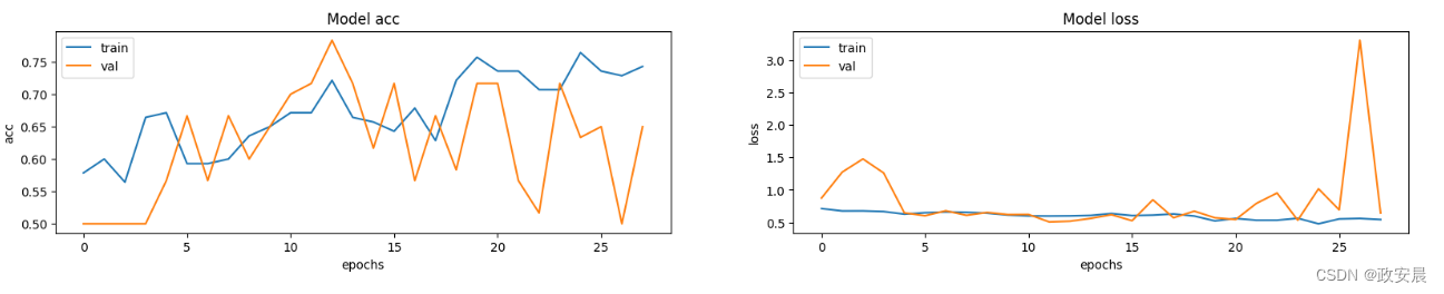
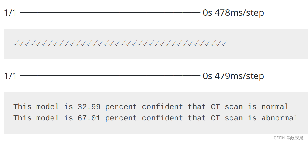
通过一次 CT 扫描进行预测
# Load best weights.
model.load_weights("3d_image_classification.keras")
prediction = model.predict(np.expand_dims(x_val[0], axis=0))[0]
scores = [1 - prediction[0], prediction[0]]

class_names = ["normal", "abnormal"]
for score, name in zip(scores, class_names):
    print(
        "This model is %.2f percent confident that CT scan is %s"
        % ((100 * score), name)
    )
演绎展示: