目录
数据收集
导入
定义超参数
加载数据
可视化数据
准备数据生成器
定义增强变换
创建训练和验证分割
数据生成器调查
模型构建
模型编译和训练
进行预测并将其可视化
更进一步
政安晨的个人主页:政安晨
欢迎 👍点赞✍评论⭐收藏
收录专栏: TensorFlow与Keras机器学习实战
希望政安晨的博客能够对您有所裨益,如有不足之处,欢迎在评论区提出指正!
本文目标:利用数据增强和迁移学习训练关键点检测器。
关键点检测包括对物体关键部位的定位。例如,人脸的关键部位包括鼻尖、眉毛、眼角等。这些部分有助于以特征丰富的方式表示底层对象。关键点检测的应用包括姿势估计、人脸检测等。
在本例中,我们将使用斯坦福 Extra 数据集,利用迁移学习建立一个关键点检测器。
本示例需要 TensorFlow 2.4 或更高版本,以及 imgaug 库,可使用以下命令安装:
!pip install -q -U imgaug数据收集
StanfordExtra 数据集包含 12,000 张狗的图像以及关键点和分割图。该数据集由斯坦福狗数据集发展而来。
可通过以下命令下载:
!wget -q http://vision.stanford.edu/aditya86/ImageNetDogs/images.tar注释在 StanfordExtra 数据集中以单个 JSON 文件的形式提供,用户需要填写此表格才能访问该文件。
作者明确指示用户不要共享 JSON 文件,本示例也尊重这一愿望:您应自行获取 JSON 文件。
JSON 文件的本地版本为 stanfordextra_v12.zip。
下载文件后,我们可以解压缩。
!tar xf images.tar
!unzip -qq ~/stanfordextra_v12.zip
导入
from keras import layers
import keras

from imgaug.augmentables.kps import KeypointsOnImage
from imgaug.augmentables.kps import Keypoint
import imgaug.augmenters as iaa

from PIL import Image
from sklearn.model_selection import train_test_split
from matplotlib import pyplot as plt
import pandas as pd
import numpy as np
import json
import os
定义超参数
IMG_SIZE = 224
BATCH_SIZE = 64
EPOCHS = 5
NUM_KEYPOINTS = 24 * 2  # 24 pairs each having x and y coordinates
加载数据
作者还提供了一个元数据文件,其中指定了有关关键点的其他信息,如颜色信息、动物姿势名称等。我们将在 pandas 数据框中加载该文件,以提取信息用于可视化目的。
IMG_DIR = "Images"
JSON = "StanfordExtra_V12/StanfordExtra_v12.json"
KEYPOINT_DEF = (
    "https://github.com/benjiebob/StanfordExtra/raw/master/keypoint_definitions.csv"
)

# Load the ground-truth annotations.
with open(JSON) as infile:
    json_data = json.load(infile)

# Set up a dictionary, mapping all the ground-truth information
# with respect to the path of the image.
json_dict = {i["img_path"]: i for i in json_data}
json_dict 的单个条目如下所示:
'n02085782-Japanese_spaniel/n02085782_2886.jpg':
{'img_bbox': [205, 20, 116, 201],
 'img_height': 272,
 'img_path': 'n02085782-Japanese_spaniel/n02085782_2886.jpg',
 'img_width': 350,
 'is_multiple_dogs': False,
 'joints': [[108.66666666666667, 252.0, 1],
            [147.66666666666666, 229.0, 1],
            [163.5, 208.5, 1],
            [0, 0, 0],
            [0, 0, 0],
            [0, 0, 0],
            [54.0, 244.0, 1],
            [77.33333333333333, 225.33333333333334, 1],
            [79.0, 196.5, 1],
            [0, 0, 0],
            [0, 0, 0],
            [0, 0, 0],
            [0, 0, 0],
            [0, 0, 0],
            [150.66666666666666, 86.66666666666667, 1],
            [88.66666666666667, 73.0, 1],
            [116.0, 106.33333333333333, 1],
            [109.0, 123.33333333333333, 1],
            [0, 0, 0],
            [0, 0, 0],
            [0, 0, 0],
            [0, 0, 0],
            [0, 0, 0],
            [0, 0, 0]],
 'seg': ...}
在这个例子中,我们感兴趣的键是:
img_path
joints
关节中总共有 24 个条目。
每个条目有 3 个值:
x 坐标
y 坐标
关键点的可见性标志(1 表示可见,0 表示不可见)
我们可以看到,关节点包含多个 [0, 0, 0] 条目,表示这些关键点没有被标记。
在本例中,我们将同时考虑非可见和未标记的关键点,以便进行迷你批量学习。
# Load the metdata definition file and preview it.
keypoint_def = pd.read_csv(KEYPOINT_DEF)
keypoint_def.head()

# Extract the colours and labels.
colours = keypoint_def["Hex colour"].values.tolist()
colours = ["#" + colour for colour in colours]
labels = keypoint_def["Name"].values.tolist()


# Utility for reading an image and for getting its annotations.
def get_dog(name):
    data = json_dict[name]
    img_data = plt.imread(os.path.join(IMG_DIR, data["img_path"]))
    # If the image is RGBA convert it to RGB.
    if img_data.shape[-1] == 4:
        img_data = img_data.astype(np.uint8)
        img_data = Image.fromarray(img_data)
        img_data = np.array(img_data.convert("RGB"))
    data["img_data"] = img_data

    return data
可视化数据
现在,我们编写一个实用程序来可视化图像及其关键点。
# Parts of this code come from here:
# https://github.com/benjiebob/StanfordExtra/blob/master/demo.ipynb
def visualize_keypoints(images, keypoints):
    fig, axes = plt.subplots(nrows=len(images), ncols=2, figsize=(16, 12))
    [ax.axis("off") for ax in np.ravel(axes)]

    for (ax_orig, ax_all), image, current_keypoint in zip(axes, images, keypoints):
        ax_orig.imshow(image)
        ax_all.imshow(image)

        # If the keypoints were formed by `imgaug` then the coordinates need
        # to be iterated differently.
        if isinstance(current_keypoint, KeypointsOnImage):
            for idx, kp in enumerate(current_keypoint.keypoints):
                ax_all.scatter(
                    [kp.x],
                    [kp.y],
                    c=colours[idx],
                    marker="x",
                    s=50,
                    linewidths=5,
                )
        else:
            current_keypoint = np.array(current_keypoint)
            # Since the last entry is the visibility flag, we discard it.
            current_keypoint = current_keypoint[:, :2]
            for idx, (x, y) in enumerate(current_keypoint):
                ax_all.scatter([x], [y], c=colours[idx], marker="x", s=50, linewidths=5)

    plt.tight_layout(pad=2.0)
    plt.show()


# Select four samples randomly for visualization.
samples = list(json_dict.keys())
num_samples = 4
selected_samples = np.random.choice(samples, num_samples, replace=False)

images, keypoints = [], []

for sample in selected_samples:
    data = get_dog(sample)
    image = data["img_data"]
    keypoint = data["joints"]

    images.append(image)
    keypoints.append(keypoint)

visualize_keypoints(images, keypoints)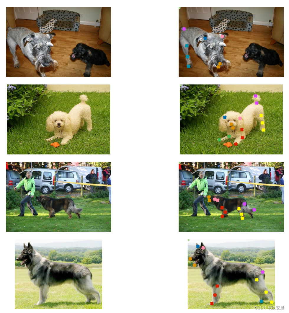
从图中可以看出,我们的图像大小并不均匀,这在现实世界的大多数情况下都是意料之中的。
但是,如果我们将这些图像的大小调整为统一形状(例如 (224 x 224)),它们的地面实况注释也会受到影响。
如果我们对图像进行任何几何变换(例如水平翻转),情况也是一样。幸运的是,imgaug 提供了可以处理这个问题的实用程序。
在后文中,我们将编写一个继承 keras.utils.Sequence 类的数据生成器,使用 imgaug 对成批数据进行数据增强。
准备数据生成器
class KeyPointsDataset(keras.utils.PyDataset):
    def __init__(self, image_keys, aug, batch_size=BATCH_SIZE, train=True, **kwargs):
        super().__init__(**kwargs)
        self.image_keys = image_keys
        self.aug = aug
        self.batch_size = batch_size
        self.train = train
        self.on_epoch_end()

    def __len__(self):
        return len(self.image_keys) // self.batch_size

    def on_epoch_end(self):
        self.indexes = np.arange(len(self.image_keys))
        if self.train:
            np.random.shuffle(self.indexes)

    def __getitem__(self, index):
        indexes = self.indexes[index * self.batch_size : (index + 1) * self.batch_size]
        image_keys_temp = [self.image_keys[k] for k in indexes]
        (images, keypoints) = self.__data_generation(image_keys_temp)

        return (images, keypoints)

    def __data_generation(self, image_keys_temp):
        batch_images = np.empty((self.batch_size, IMG_SIZE, IMG_SIZE, 3), dtype="int")
        batch_keypoints = np.empty(
            (self.batch_size, 1, 1, NUM_KEYPOINTS), dtype="float32"
        )

        for i, key in enumerate(image_keys_temp):
            data = get_dog(key)
            current_keypoint = np.array(data["joints"])[:, :2]
            kps = []

            # To apply our data augmentation pipeline, we first need to
            # form Keypoint objects with the original coordinates.
            for j in range(0, len(current_keypoint)):
                kps.append(Keypoint(x=current_keypoint[j][0], y=current_keypoint[j][1]))

            # We then project the original image and its keypoint coordinates.
            current_image = data["img_data"]
            kps_obj = KeypointsOnImage(kps, shape=current_image.shape)

            # Apply the augmentation pipeline.
            (new_image, new_kps_obj) = self.aug(image=current_image, keypoints=kps_obj)
            batch_images[i,] = new_image

            # Parse the coordinates from the new keypoint object.
            kp_temp = []
            for keypoint in new_kps_obj:
                kp_temp.append(np.nan_to_num(keypoint.x))
                kp_temp.append(np.nan_to_num(keypoint.y))

            # More on why this reshaping later.
            batch_keypoints[i,] = np.array(kp_temp).reshape(1, 1, 24 * 2)

        # Scale the coordinates to [0, 1] range.
        batch_keypoints = batch_keypoints / IMG_SIZE

        return (batch_images, batch_keypoints)
要进一步了解如何在 imgaug 中使用关键点,请查看本文。
定义增强变换
train_aug = iaa.Sequential(
    [
        iaa.Resize(IMG_SIZE, interpolation="linear"),
        iaa.Fliplr(0.3),
        # `Sometimes()` applies a function randomly to the inputs with
        # a given probability (0.3, in this case).
        iaa.Sometimes(0.3, iaa.Affine(rotate=10, scale=(0.5, 0.7))),
    ]
)

test_aug = iaa.Sequential([iaa.Resize(IMG_SIZE, interpolation="linear")])
创建训练和验证分割
np.random.shuffle(samples)
train_keys, validation_keys = (
    samples[int(len(samples) * 0.15) :],
    samples[: int(len(samples) * 0.15)],
)
数据生成器调查
train_dataset = KeyPointsDataset(
    train_keys, train_aug, workers=2, use_multiprocessing=True
)
validation_dataset = KeyPointsDataset(
    validation_keys, test_aug, train=False, workers=2, use_multiprocessing=True
)

print(f"Total batches in training set: {len(train_dataset)}")
print(f"Total batches in validation set: {len(validation_dataset)}")

sample_images, sample_keypoints = next(iter(train_dataset))
assert sample_keypoints.max() == 1.0
assert sample_keypoints.min() == 0.0

sample_keypoints = sample_keypoints[:4].reshape(-1, 24, 2) * IMG_SIZE
visualize_keypoints(sample_images[:4], sample_keypoints)
演绎展示:
Total batches in training set: 166
Total batches in validation set: 29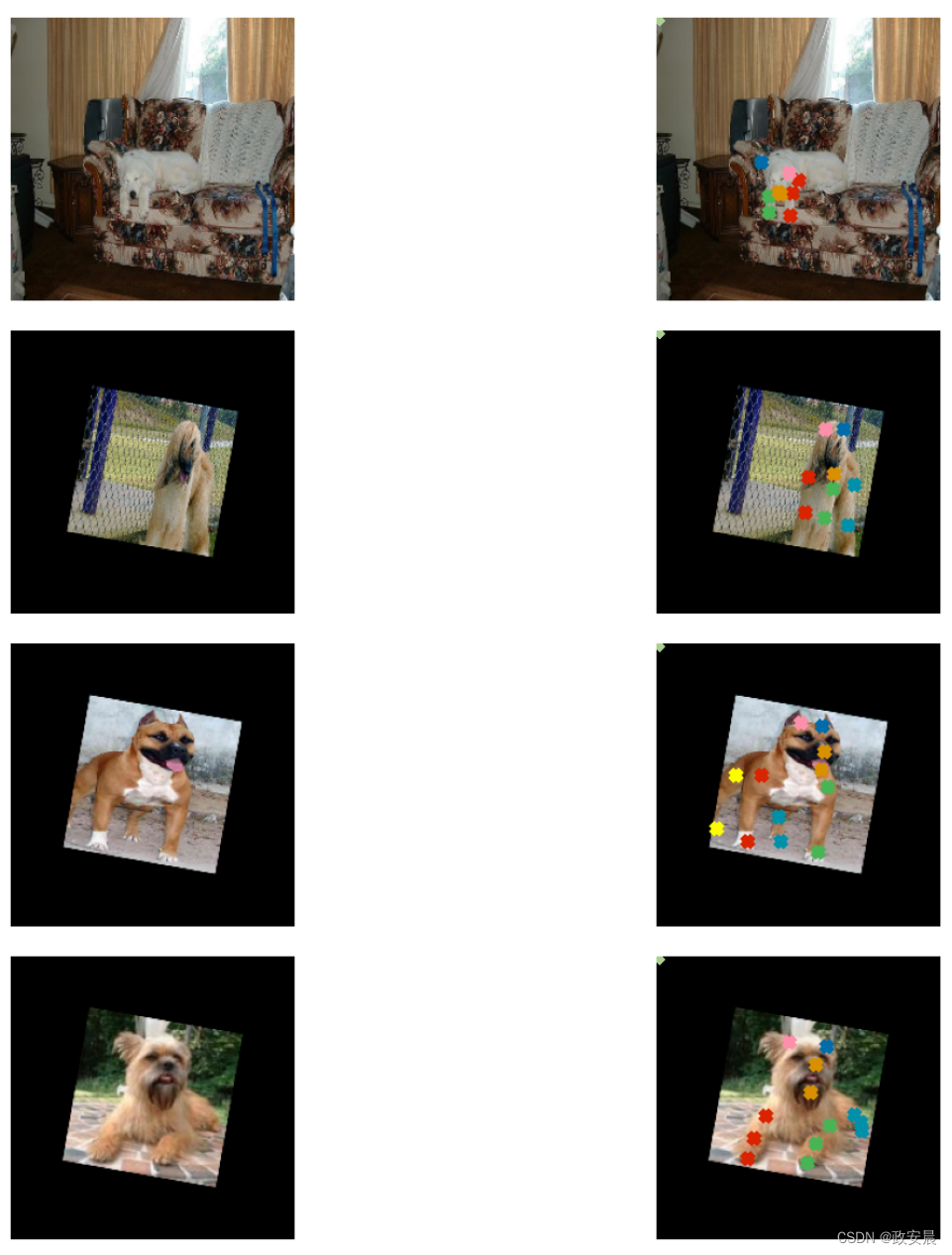
模型构建
Stanford dogs 数据集(StanfordExtra 数据集基于该数据集)是使用 ImageNet-1k 数据集构建的。因此,在 ImageNet-1k 数据集上预训练的模型很可能对这项任务有用。我们将使用在该数据集上预先训练好的 MobileNetV2 作为骨干,从图像中提取有意义的特征,然后将这些特征传递给自定义回归头用于预测坐标。
def get_model():
    # Load the pre-trained weights of MobileNetV2 and freeze the weights
    backbone = keras.applications.MobileNetV2(
        weights="imagenet",
        include_top=False,
        input_shape=(IMG_SIZE, IMG_SIZE, 3),
    )
    backbone.trainable = False

    inputs = layers.Input((IMG_SIZE, IMG_SIZE, 3))
    x = keras.applications.mobilenet_v2.preprocess_input(inputs)
    x = backbone(x)
    x = layers.Dropout(0.3)(x)
    x = layers.SeparableConv2D(
        NUM_KEYPOINTS, kernel_size=5, strides=1, activation="relu"
    )(x)
    outputs = layers.SeparableConv2D(
        NUM_KEYPOINTS, kernel_size=3, strides=1, activation="sigmoid"
    )(x)

    return keras.Model(inputs, outputs, name="keypoint_detector")
我们定制的网络是全卷积网络,因此与具有全连接密集层的相同版本网络相比,它对参数更加友好。
get_model().summary()演绎展示:
Downloading data from https://storage.googleapis.com/tensorflow/keras-applications/mobilenet_v2/mobilenet_v2_weights_tf_dim_ordering_tf_kernels_1.0_224_no_top.h5
 9406464/9406464 ━━━━━━━━━━━━━━━━━━━━ 0s 0us/step
请注意网络的输出形状:(None, 1, 1, 48)。
这就是我们重塑坐标的原因:batch_keypoints[i, :] = np.array(kp_temp).reshape(1, 1, 24 * 2)。
模型编译和训练
在本例中,我们只对网络进行 5 个历元的训练。
model = get_model()
model.compile(loss="mse", optimizer=keras.optimizers.Adam(1e-4))
model.fit(train_dataset, validation_data=validation_dataset, epochs=EPOCHS)
Epoch 1/5
166/166 ━━━━━━━━━━━━━━━━━━━━ 84s 415ms/step - loss: 0.1110 - val_loss: 0.0959
Epoch 2/5
166/166 ━━━━━━━━━━━━━━━━━━━━ 79s 472ms/step - loss: 0.0874 - val_loss: 0.0802
Epoch 3/5
166/166 ━━━━━━━━━━━━━━━━━━━━ 78s 463ms/step - loss: 0.0789 - val_loss: 0.0765
Epoch 4/5
166/166 ━━━━━━━━━━━━━━━━━━━━ 78s 467ms/step - loss: 0.0769 - val_loss: 0.0731
Epoch 5/5
166/166 ━━━━━━━━━━━━━━━━━━━━ 77s 464ms/step - loss: 0.0753 - val_loss: 0.0712
<keras.src.callbacks.history.History at 0x7fb5c4299ae0>进行预测并将其可视化
sample_val_images, sample_val_keypoints = next(iter(validation_dataset))
sample_val_images = sample_val_images[:4]
sample_val_keypoints = sample_val_keypoints[:4].reshape(-1, 24, 2) * IMG_SIZE
predictions = model.predict(sample_val_images).reshape(-1, 24, 2) * IMG_SIZE

# Ground-truth
visualize_keypoints(sample_val_images, sample_val_keypoints)

# Predictions
visualize_keypoints(sample_val_images, predictions)
演绎展示:
1/1 ━━━━━━━━━━━━━━━━━━━━ 7s 7s/step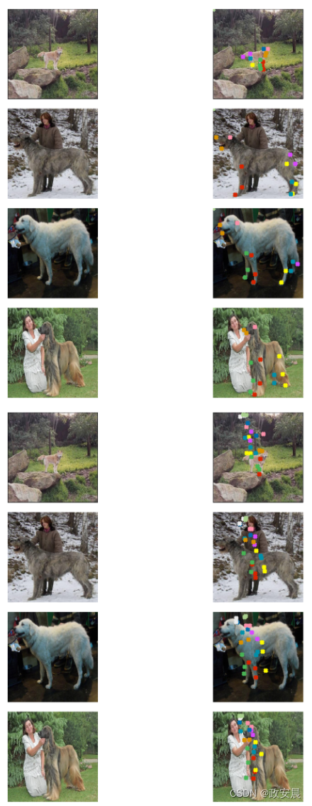
通过更多的训练,预测结果可能会有所改善。
更进一步
尝试使用 imgaug 的其他增强变换,研究其对结果的影响。
在这里,我们从预训练网络中线性转移了特征,也就是说,我们没有对其进行微调。
我们鼓励你在这项任务中对其进行微调,看看是否能提高性能。您还可以尝试不同的架构,看看它们对最终性能有什么影响。
![Amazon云计算AWS之[1]基础存储架构Dynamo](https://img-blog.csdnimg.cn/direct/0bd82ce343354d1a9881ebbfd7443378.png#pic_center)