文章目录
- CS224N: 作业2 word2vec (49 Points)
- 1. Math: 理解 word2vec
- 计算 J n a i v e − s o f t m a x ( v c , o , U ) J_{naive-softmax}(v_c, o, U) Jnaive−softmax(vc,o,U) 关于 v c v_c vc 的偏导数
- 计算 J n a i v e − s o f t m a x ( v c , o , U ) J_{naive-softmax}(v_c, o, U) Jnaive−softmax(vc,o,U) 关于每一个 u w u_w uw 的偏导数
- 计算 The Leaky ReLU (Leaky Rectified Linear Unit) 的导函数
- 计算 sigmoid function 的导函数
- The Negative Sampling loss
- 2. Code: 实现 word2vec
CS224N: 作业2 word2vec (49 Points)
1. Math: 理解 word2vec
word2vec 的关键思想是: a word is known by the company it keeps.
给定一个中心词
c
c
c, 一个大小为
n
n
n 的窗口, 那么相对于
c
c
c 的上下文就是
O
O
O, 例如在文本: ... problems turning into banking crises as ... 中, 若
c
c
c 为 banking,
n
=
2
n=2
n=2, 则
O
O
O 为 turning into crises as 这4个单词.
因此, Skip-gram word2vec 的目的就是学习一个概率分布: P ( O ∣ C ) P(O|C) P(O∣C). 特别的, 对于一个特定的中心词 c c c 和一个特定的上下文单词 o o o, 我们有: P ( O = o ∣ C = c ) = exp ( u o T v c ) Σ w ∈ V o c a b exp ( u w T v c ) P(O=o|C=c)=\frac{\exp{(u_o^Tv_c)}}{\Sigma_{w\in Vocab}\exp{(u_w^Tv_c)}} P(O=o∣C=c)=Σw∈Vocabexp(uwTvc)exp(uoTvc)
这里, Vocab 是指词汇表, 它的长度为 N. 定义两个矩阵 U 和 V, U 表示 outside word vectors, 大小为 (D, N), 也即该矩阵的列向量
U
i
U_i
Ui 表示词表第 i 个单词的词向量, 词向量维数是 D. V 矩阵大小与 U 相同, 但他表示每个单词作为中心词时的词向量矩阵.
接下来根据优化目标来定义损失函数.
对于特定的
c
c
c和
o
o
o, 它的损失贡献是:
J
n
a
i
v
e
−
s
o
f
t
m
a
x
(
v
c
,
o
,
U
)
=
−
log
P
(
O
=
o
∣
C
=
c
)
J_{naive-softmax}(v_c, o, U) = −\log{P(O = o|C = c)}
Jnaive−softmax(vc,o,U)=−logP(O=o∣C=c)
这可以视为 真实分布
y
y
y 与 预测分布
y
^
\hat{y}
y^ 之间的交叉熵损失(对于特定的
c
c
c和
o
o
o), 这里
y
y
y和
y
^
\hat{y}
y^为N维向量, 第 k 个分量表示词汇表第k个词是指定中心词
c
c
c的 outside word 的条件概率.
y
y
y 是一个 one-hot 向量, 它在实际 outside word 的分量处为1, 其它地方是0.
y
^
\hat{y}
y^ 由
P
(
O
∣
C
=
c
)
P(O|C=c)
P(O∣C=c) 给出. 因此很容易就能看出该损失函数实际上就是真实分布
y
y
y 与 预测分布
y
^
\hat{y}
y^ 之间的交叉熵损失
插播一条定义, 交叉熵的定义是:
- Cross-Entropy Loss
Thecross-entropy lossbetween the true (discrete) probability distribution p p p and another distribution q q q is: − Σ i p i l o g ( q i ) -\Sigma_{i}p_ilog(q_i) −Σipilog(qi)
计算 J n a i v e − s o f t m a x ( v c , o , U ) J_{naive-softmax}(v_c, o, U) Jnaive−softmax(vc,o,U) 关于 v c v_c vc 的偏导数
结果只能使用
y
y
y 和
y
^
\hat{y}
y^ 以及
U
U
U 来表示, 请给出详细计算过程
∂
(
J
)
∂
(
v
c
)
=
∂
∂
(
v
c
)
(
−
log
P
(
O
=
o
∣
C
=
c
)
)
=
∂
∂
(
v
c
)
(
log
∑
u
w
∈
V
o
c
a
b
(
exp
u
w
T
v
c
)
−
u
o
T
v
c
)
=
−
u
o
+
1
∑
u
w
∈
V
o
c
a
b
(
exp
u
w
T
v
c
)
∂
∂
(
v
c
)
∑
u
w
∈
V
o
c
a
b
(
exp
u
w
T
v
c
)
=
−
u
o
+
∑
u
w
∈
V
o
c
a
b
(
exp
u
w
T
v
c
)
u
w
∑
u
x
∈
V
o
c
a
b
(
exp
u
x
T
v
c
)
=
−
u
o
+
∑
u
w
∈
V
o
c
a
b
(
exp
u
w
T
v
c
)
∑
u
x
∈
V
o
c
a
b
(
exp
u
x
T
v
c
)
u
w
=
−
u
o
+
∑
u
w
∈
V
o
c
a
b
P
(
O
=
w
∣
C
=
c
)
u
w
=
−
u
o
+
∑
u
w
∈
V
o
c
a
b
y
w
^
u
w
=
−
u
o
+
U
y
^
=
U
(
y
^
−
y
)
\begin{align*} \frac{\partial(J)}{\partial(v_c)} & = \frac{\partial}{\partial(v_c)}{(−\log P(O = o|C = c))} \\ & =\frac{\partial}{\partial(v_c)}(\log \sum_{u_w\in Vocab}(\exp{u_w^Tv_c})-u_o^Tv_c) \\ & = -u_o + \frac{1}{\sum_{u_w\in Vocab}(\exp{u_w^Tv_c})}\frac{\partial}{\partial(v_c)}\sum_{u_w\in Vocab}(\exp{u_w^Tv_c}) \\ & = -u_o + \frac{\sum_{u_w\in Vocab}(\exp{u_w^Tv_c})u_w}{\sum_{u_x\in Vocab}(\exp{u_x^Tv_c})} \\ & = -u_o + \sum_{u_w\in Vocab}\frac{(\exp{u_w^Tv_c})}{\sum_{u_x\in Vocab}(\exp{u_x^Tv_c})}u_w \\ & = -u_o + \sum_{u_w\in Vocab}P(O=w|C=c)u_w \\ & = -u_o + \sum_{u_w\in Vocab}\hat{y_w}u_w \\ & = -u_o + U\hat{y} = U(\hat{y}-y) \end{align*}
∂(vc)∂(J)=∂(vc)∂(−logP(O=o∣C=c))=∂(vc)∂(loguw∈Vocab∑(expuwTvc)−uoTvc)=−uo+∑uw∈Vocab(expuwTvc)1∂(vc)∂uw∈Vocab∑(expuwTvc)=−uo+∑ux∈Vocab(expuxTvc)∑uw∈Vocab(expuwTvc)uw=−uo+uw∈Vocab∑∑ux∈Vocab(expuxTvc)(expuwTvc)uw=−uo+uw∈Vocab∑P(O=w∣C=c)uw=−uo+uw∈Vocab∑yw^uw=−uo+Uy^=U(y^−y)
-
When is the gradient you computed equal to zero?
也即 $ U(\hat{y}-y)=0 $, 这是齐次线性方程组, 矩阵的行秩小于列秩, 此时方程组有无数解. -
计算得到的结果表现形式是一个差值的形式, 给出解释为什么当 v c v_c vc 减去这个偏导数后会提升 v c v_c vc 的表现.
计算 J n a i v e − s o f t m a x ( v c , o , U ) J_{naive-softmax}(v_c, o, U) Jnaive−softmax(vc,o,U) 关于每一个 u w u_w uw 的偏导数
对上下文词向量
u
w
u_w
uw求导
∂
(
J
)
∂
(
u
w
)
=
∂
∂
(
u
w
)
(
−
log
P
(
O
=
o
∣
C
=
c
)
)
=
∂
∂
(
u
w
)
log
∑
u
w
∈
V
o
c
a
b
(
exp
u
w
T
v
c
)
−
∂
∂
(
u
w
)
u
o
T
v
c
\begin{align*} \frac{\partial(J)}{\partial(u_w)} &= \frac{\partial}{\partial(u_w)}{(−\log P(O = o|C = c))} \\ &= \frac{\partial}{\partial(u_w)}\log \sum_{u_w\in Vocab}(\exp{u_w^Tv_c})-\frac{\partial}{\partial(u_w)}u_o^Tv_c \end{align*}
∂(uw)∂(J)=∂(uw)∂(−logP(O=o∣C=c))=∂(uw)∂loguw∈Vocab∑(expuwTvc)−∂(uw)∂uoTvc
分为两部分计算, 对于前一部分 PartA:
p
a
r
t
A
=
exp
u
w
T
v
c
∑
u
w
∈
V
o
c
a
b
(
exp
u
w
T
v
c
)
v
c
=
P
(
O
=
w
∣
C
=
c
)
v
c
=
y
w
^
v
c
\begin{matrix} partA &=& \frac{\exp{u_w^Tv_c}}{\sum_{u_w\in Vocab}(\exp{u_w^Tv_c})}v_c=P(O=w|C=c)v_c=\hat{y_w}v_c \end{matrix}
partA=∑uw∈Vocab(expuwTvc)expuwTvcvc=P(O=w∣C=c)vc=yw^vc
对于后一个部分, 当 w 不等于 o 时, partB=0, 否则等于
v
c
v_c
vc, 因此:
∂
(
J
)
∂
(
u
w
)
=
(
y
^
w
−
y
w
)
v
c
\frac{\partial(J)}{\partial(u_w)}=(\hat{y}_w-y_w)v_c
∂(uw)∂(J)=(y^w−yw)vc
- 计算
J
n
a
i
v
e
−
s
o
f
t
m
a
x
(
v
c
,
o
,
U
)
J_{naive-softmax}(v_c, o, U)
Jnaive−softmax(vc,o,U) 关于
U
U
U 的偏导数(也即把上面的结果表示为矩阵形式)
∂ ( J ) ∂ ( U ) = ⟨ ∂ ∂ ( u 1 ) , ∂ ∂ ( u 2 ) , … , ∂ ∂ ( u N ) ⟩ \begin{matrix} \frac{\partial(J)}{\partial(U)} & = \braket{\frac{\partial}{\partial(u_1)}, \frac{\partial}{\partial(u_2)}, \dots, \frac{\partial}{\partial(u_N)}} \end{matrix} ∂(U)∂(J)=⟨∂(u1)∂,∂(u2)∂,…,∂(uN)∂⟩
计算 The Leaky ReLU (Leaky Rectified Linear Unit) 的导函数
f
(
x
)
=
max
(
α
x
,
x
)
(
0
<
α
<
1
)
f(x) = \max(\alpha x, x) (0<\alpha<1)
f(x)=max(αx,x)(0<α<1)
d
d
x
f
(
x
)
=
{
α
,
x
<
=
0
1
,
x
>
0
\frac{d}{dx}f(x)= \begin{cases} \alpha, &x<=0 \\ 1, &x>0 \end{cases}
dxdf(x)={α,1,x<=0x>0
计算 sigmoid function 的导函数
σ
(
x
)
=
1
1
+
e
−
x
\sigma(x) = \frac{1}{1+e^{-x}}
σ(x)=1+e−x1
σ
′
(
x
)
=
−
1
(
1
+
e
−
x
)
2
∗
(
−
e
−
x
)
=
e
−
x
(
1
+
e
−
x
)
2
=
σ
(
x
)
(
1
−
σ
(
x
)
)
\sigma'(x) = -\frac{1}{(1+e^{-x})^2}*(-e^{-x})=\frac{e^{-x}}{(1+e^{-x})^2}=\sigma(x)(1-\sigma(x))
σ′(x)=−(1+e−x)21∗(−e−x)=(1+e−x)2e−x=σ(x)(1−σ(x))
The Negative Sampling loss
考虑负采样的损失函数, 它是原生 softmax 损失的替代版, 假设先从词表中随机挑选 N 个负样本(单词), 标记为
w
1
,
w
2
,
…
,
w
K
w_1, w_2, \dots, w_K
w1,w2,…,wK, 它们的 outside vectors 是:
u
1
,
u
1
,
…
,
u
K
u_1, u_1, \dots, u_K
u1,u1,…,uK. 注意, K个负样本互不相同, 上下文单词 o 不在这K个样本中. 那么对于指定的中心词c和外部词o, 损失函数是:
J
n
e
g
−
s
a
m
p
l
e
(
v
c
,
o
,
U
)
=
−
log
(
σ
(
u
o
T
v
c
)
)
−
∑
s
=
1
K
log
(
σ
(
−
u
s
T
v
c
)
)
J_{neg-sample(v_c, o, U)} = -\log(\sigma(u_o^Tv_c))-\sum_{s=1}^K \log{(\sigma(-u_s^Tv_c))}
Jneg−sample(vc,o,U)=−log(σ(uoTvc))−s=1∑Klog(σ(−usTvc))
- 计算 J 关于 v c v_c vc, u s u_s us 的偏导. 结果使用 v c v_c vc, u o u_o uo, u w s u_{w_s} uws来表达.
- 依据链式求导法则, 反向传播算法在计算偏导时可以利用先前的计算以节省时间开销, 请结合偏导计算过程给出说明. 注意, 你可以使用如下符号: U o , { w 1 , … , w K } = [ u o , − u 1 , … , − u K ] U_{o,{\{w_1, \dots, w_K\}}}=[u_o, -u_1,\dots,-u_K] Uo,{w1,…,wK}=[uo,−u1,…,−uK] 和向量 1 \bf{1} 1(包含K+1个1).
- 请用一句话说明为什么负采样损失要比原来的softmax损失更高效.
∂
(
J
)
∂
(
v
c
)
=
∂
∂
(
v
c
)
(
−
log
(
σ
(
u
o
T
v
c
)
)
)
+
∂
(
J
)
∂
(
v
c
)
(
−
∑
s
=
1
K
log
(
σ
(
−
u
s
T
v
c
)
)
)
=
A
+
B
\begin{align*} \frac{\partial(J)}{\partial(v_c)} &= \frac{\partial}{\partial(v_c)}(-\log(\sigma(u_o^Tv_c))) + \frac{\partial(J)}{\partial(v_c)}(-\sum_{s=1}^K{\log(\sigma(-u_s^Tv_c))}) \\ &=A+B \end{align*}
∂(vc)∂(J)=∂(vc)∂(−log(σ(uoTvc)))+∂(vc)∂(J)(−s=1∑Klog(σ(−usTvc)))=A+B
计算 A:
A
=
−
1
σ
(
u
o
T
v
c
)
∗
(
1
−
σ
(
u
o
T
v
c
)
)
σ
(
u
o
T
v
c
)
∗
u
o
=
(
σ
(
u
o
T
v
c
)
−
1
)
u
o
\begin{align*} A&=\frac{-1}{\sigma(u_o^Tv_c)}*(1-\sigma(u_o^Tv_c))\sigma(u_o^Tv_c)*u_o \\ &=(\sigma(u_o^Tv_c)-1)u_o \end{align*}
A=σ(uoTvc)−1∗(1−σ(uoTvc))σ(uoTvc)∗uo=(σ(uoTvc)−1)uo
计算 B:
B
=
∑
s
=
1
K
−
1
σ
(
−
u
s
T
v
c
)
∗
σ
(
−
u
s
T
v
c
)
(
1
−
σ
(
−
u
s
T
v
c
)
)
∗
(
−
u
s
)
=
∑
s
=
1
K
(
1
−
σ
(
−
u
s
T
v
c
)
)
u
s
\begin{align*} B&=\sum_{s=1}^K\frac{-1}{\sigma(-u_s^Tv_c)}*{\sigma(-u_s^Tv_c)}(1-\sigma(-u_s^Tv_c))*(-u_s)\\ &=\sum_{s=1}^K(1-\sigma(-u_s^Tv_c))u_s \end{align*}
B=s=1∑Kσ(−usTvc)−1∗σ(−usTvc)(1−σ(−usTvc))∗(−us)=s=1∑K(1−σ(−usTvc))us
因此:
∂
(
J
)
∂
(
v
c
)
=
(
σ
(
u
o
T
v
c
)
−
1
)
u
o
+
∑
s
=
1
K
(
1
−
σ
(
−
u
s
T
v
c
)
)
u
s
\begin{align*} \frac{\partial(J)}{\partial(v_c)} &=(\sigma(u_o^Tv_c)-1)u_o+\sum_{s=1}^K(1-\sigma(-u_s^Tv_c))u_s \end{align*}
∂(vc)∂(J)=(σ(uoTvc)−1)uo+s=1∑K(1−σ(−usTvc))us
计算 J 关于
u
s
u_s
us 的偏导数:
∂
(
J
)
∂
(
u
s
)
=
∂
∂
(
u
s
)
(
−
log
(
σ
(
u
o
T
v
c
)
)
)
+
∂
(
J
)
∂
(
u
s
)
(
−
∑
k
=
1
K
log
(
σ
(
−
u
k
T
v
c
)
)
)
=
−
1
σ
(
−
u
s
T
v
c
)
∗
σ
(
−
u
s
T
v
c
)
(
1
−
σ
(
−
u
s
T
v
c
)
)
∗
(
−
v
c
)
=
(
1
−
σ
(
−
u
s
T
v
c
)
)
v
c
\begin{align*} \frac{\partial(J)}{\partial(u_s)} &= \frac{\partial}{\partial(u_s)}(-\log(\sigma(u_o^Tv_c))) + \frac{\partial(J)}{\partial(u_s)}(-\sum_{k=1}^K{\log(\sigma(-u_k^Tv_c))}) \\ &= \frac{-1}{\sigma(-u_s^Tv_c)}*{\sigma(-u_s^Tv_c)}(1-\sigma(-u_s^Tv_c))*(-v_c) \\ &= (1-\sigma(-u_s^Tv_c))v_c \end{align*}
∂(us)∂(J)=∂(us)∂(−log(σ(uoTvc)))+∂(us)∂(J)(−k=1∑Klog(σ(−ukTvc)))=σ(−usTvc)−1∗σ(−usTvc)(1−σ(−usTvc))∗(−vc)=(1−σ(−usTvc))vc
计算 J 关于
u
o
u_o
uo 的偏导数:
∂
(
J
)
∂
(
u
o
)
=
∂
∂
(
u
o
)
(
−
log
(
σ
(
u
o
T
v
c
)
)
)
=
(
σ
(
u
o
T
v
c
)
−
1
)
v
c
\begin{align*} \frac{\partial(J)}{\partial(u_o)} &= \frac{\partial}{\partial(u_o)}(-\log(\sigma(u_o^Tv_c))) \\ &= (\sigma(u_o^Tv_c)-1)v_c \end{align*}
∂(uo)∂(J)=∂(uo)∂(−log(σ(uoTvc)))=(σ(uoTvc)−1)vc
- 负采样loss在计算导数时不需要遍历整个词表, 只需要K个负样本.
2. Code: 实现 word2vec
在这一部分,将实现word2vec模型,并使用随机梯度下降( SGD )训练自己的词向量。在开始之前,首先在任务目录内运行以下命令,以便创建合适的conda虚拟环境。这就保证了你有完成任务所必需的所有包。还需要注意的是,您可能希望在编写代码之前完成前面的数学部分,因为您将被要求在Python中实现数学函数。你可能会想按顺序实施和测试这一部分的每一部分,因为问题是循序渐进的。
对于每个需要实现的方法,我们在代码注释中包含了我们的解决方案大约有多少行代码。这些数字都包含在里面,用来指导你。你不必拘泥于它们,你可以随心所欲地编写更短或更长的代码。如果你认为你的实现比我们的实现长得多,那就表明你可以使用一些numpy方法来使你的代码既短又快。因为Python中的循环在使用大型数组时需要很长的时间才能完成,所以我们期望你使用numpy方法。我们将检查您的代码的效率。当你向Gradescope提交代码时,你就能看到自动评分器的结果,我们建议尽快提交代码。
(1). 我们将从 word2vec.py 入手开始实现方法。可以通过运行 python word2vec.py m 来测试特定的方法,其中m是您想要测试的方法。例如,可以通过运行python word2vec.py sigmoid来测试sigmoid方法。
a. Implement the
sigmoidmethod, which takes in a vector and applies the sigmoid function to it.
b. Implement the softmax loss and gradient in thenaiveSoftmaxLossAndGradientmethod.
c. Implement the negative sampling loss and gradient in thenegSamplingLossAndGradientmethod.
d. Implement the skip-gram model in theskipgrammethod
When you are done, test your entire implementation by running python word2vec.py
(2). Complete the implementation for your SGD optimizer in the sgd method of sgd.py. Test your implementation by running python sgd.py
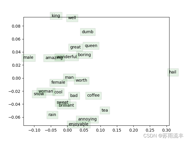
(3). 展示时间!现在我们要加载一些真实的数据,用你刚实现的一切来训练词向量!我们将使用Stanford Sentiment树库( SST )数据集来训练词向量,并将其应用到一个简单的情感分析任务中。首先需要获取数据集,为此,运行sh get dataset.sh。对于该部分没有额外编写的代码;只需运行 python run.py. 经过40,000次迭代后,脚本将完成,并出现一个词向量的可视化。也会以 word_vectors.png 的形式保存在项目目录中。将结果图片包含在你的作业中写出来。至多用三句话简要解释一下你在结果图片中看到的内容。这可能包括但不限于对聚类的观察和你希望聚类但没有聚类的单词。
以下贴出核心实现:
def naiveSoftmaxLossAndGradient(centerWordVec, outsideWordIdx, outsideVectors, datase):
	### YOUR CODE HERE (~6-8 Lines)
    y_hat = softmax(np.matmul(outsideVectors, centerWordVec))   # y_hat = P(O|C=c), (N,)
    y = np.zeros(y_hat.shape[0])
    y[outsideWordIdx] = 1                                       # y, one-hot vector, (N,)
    loss = -np.log(y_hat[outsideWordIdx])                       # loss = -log(y_hat[o]), scalar
    gradCenterVec = np.matmul(outsideVectors.T, y_hat-y)        # dJ/dv_c = U(y_hat-y), (D,)
    gradOutsideVecs = np.matmul((y_hat-y).reshape(-1,1), centerWordVec.reshape(1,-1))   # (N, D)
    ### END YOUR CODE
    return loss, gradCenterVec, gradOutsideVecs

def negSamplingLossAndGradient(centerWordVec, outsideWordIdx, outsideVectors, dataset, K=10):
    # Negative sampling of words is done for you. Do not modify this if you
    # wish to match the autograder and receive points!
    negSampleWordIndices = getNegativeSamples(outsideWordIdx, dataset, K)
    indices = [outsideWordIdx] + negSampleWordIndices

    ### YOUR CODE HERE (~10 Lines)
    gradCenterVec = np.zeros_like(centerWordVec)
    gradOutsideVecs = np.zeros_like(outsideVectors)
    # loss function
    loss = -np.log(sigmoid(outsideVectors[outsideWordIdx].dot(centerWordVec)))
    for idx in negSampleWordIndices:
        loss -= np.log(sigmoid(-outsideVectors[idx].dot(centerWordVec)))
    # gradient
    gradCenterVec -= (1 - sigmoid(centerWordVec.dot(outsideVectors[outsideWordIdx]))) * outsideVectors[outsideWordIdx]
    for k in negSampleWordIndices:
        gradCenterVec += (1 - sigmoid(-centerWordVec.dot(outsideVectors[k]))) * outsideVectors[k]
    gradOutsideVecs[outsideWordIdx] = -(1 - sigmoid(centerWordVec.dot(outsideVectors[outsideWordIdx]))) * centerWordVec
    for k in negSampleWordIndices:
        gradOutsideVecs[k] += (1 - sigmoid(-centerWordVec.dot(outsideVectors[k]))) * centerWordVec
    ### END YOUR CODE
    return loss, gradCenterVec, gradOutsideVecs

def skipgram(currentCenterWord, windowSize, outsideWords, word2Ind,
             centerWordVectors, outsideVectors, dataset,
             word2vecLossAndGradient=naiveSoftmaxLossAndGradient):
	loss = 0.0
    gradCenterVecs = np.zeros(centerWordVectors.shape)
    gradOutsideVectors = np.zeros(outsideVectors.shape)
    ### YOUR CODE HERE (~8 Lines)
    currentCenterIdx = word2Ind[currentCenterWord]
    for word in outsideWords:
        loss_w, grad_cv, grad_ov = word2vecLossAndGradient(
            centerWordVectors[currentCenterIdx],
            word2Ind[word],
            outsideVectors,
            dataset
        )
        loss += loss_w
        gradCenterVecs[currentCenterIdx] += grad_cv
        gradOutsideVectors += grad_ov
    ### END YOUR CODE
    return loss, gradCenterVecs, gradOutsideVectors
sgd部分:
### YOUR CODE HERE (~2 lines)
loss, grad = f(x)
x = x - step*grad
### END YOUR CODE
运行结果:
iter 39910: 9.324637
iter 39920: 9.284225
iter 39930: 9.298478
iter 39940: 9.296606
iter 39950: 9.313374
iter 39960: 9.317475
iter 39970: 9.330720
iter 39980: 9.410215
iter 39990: 9.418270
iter 40000: 9.367644
sanity check: cost at convergence should be around or below 10
training took 6372 seconds


![【饿了么笔试题汇总】[全网首发]2024-04-12-饿了么春招笔试题-三语言题解(CPP/Python/Java)](https://img-blog.csdnimg.cn/direct/60dd47443c3048618c27e2778460ffae.png#pic_center)

![[lesson20]初始化列表的使用](https://img-blog.csdnimg.cn/direct/aab952e1761943ceb67416ac8b644ff4.png#pic_center)