概述

3D-DIC is a non-contact optical-numerical technique for measuring the 3D shape and full-field displacement, deformation and strain, from stereo digital images of the surface of an object.

---

The MATLAB package is composed of four main scripts:

1. stereo camera calibration;
2. image cross-correlation (2D-DIC);
3. 3D reconstruction;
4. post-processing.

---

Algorithms and workflow

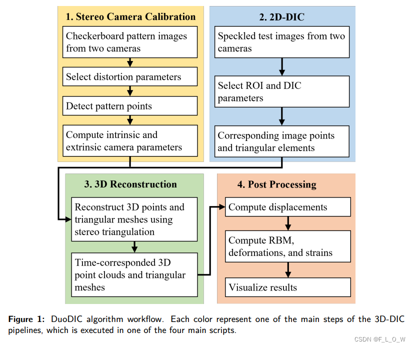
Figure 1 outlines the workflow of the 3D-DIC procedure.

The experimental setup used for taking these images consisted of
two machine-vision cameras (BFS-U3-51S5M-C, FLIR, USA), each equipped with a 5.0 MP
Sony IMX250 monochrome sensor and a 25 mm lens (Fujinon HF25SA-1, Fujifilm Corporation,
Japan).

相机由硬件触发进行同步： The cameras were synchronously hardware-triggered using a MatchID Triggerbox (MatchID, Belgium).

---

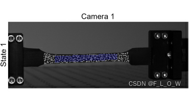
A rubber dog-bone specimen（长得像狗骨头一样的橡胶标本）, cut out of a bicycle tube, was mounted on
an optical table (Thorlabs, USA), such that its left end was fixed and its right end was moved
to the right in 19 steps with 1 mm increments, such that a total of 20 images were taken from
each camera (one reference state and 19 deformed states).

狗骨头橡胶标本示意图：

Step 1: Stereo camera calibration

使用 MathWorks Computer Vision Toolbox进行相机标定。

• 脚本的输入是：
  multiple simultaneous images of a checkerboard target captured by two cameras in a stereo pair.

---

The intrinsic parameters include focal lengths, principal point, and up to 6 distortion coefficients.

The extrinsic camera parameters comprise the 3D position and orientation of the second camera with respect to the first. Furthermore, the computed camera parameters are used for computing the reprojection errors, which represent the distance between the reprojected and the detected pattern points, and comprise the accuracy of the estimated camera parameters.

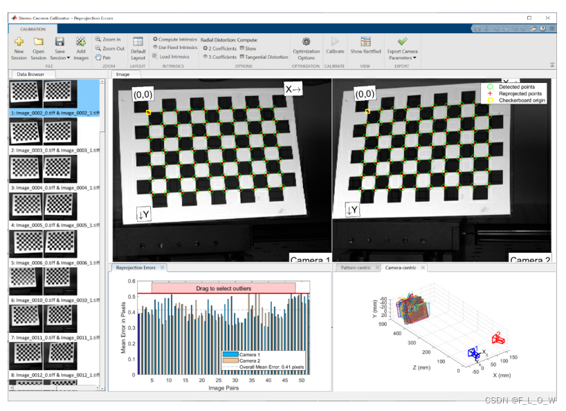
Figure 2: The top panels show the detected and reprojected points for a pair of stereo images. The bottom left panel shows the mean reprojection error for all pairs of images, and the bottom right panel shows the estimated positions and orientations of the cameras with respect to the checkerboard pattern images.

Step 2: Image cross-correlation (2D-DIC)

脚本输入： multiple images of a speckled test object captured simultaneously by the stereo camera pair.
The first image pair defines the reference configuration, to which the rest of the image are compared.

---

Ncorr toolbox is utilized in this step to detect a dense grid of matching points on all images.
Although Ncorr was created as a 2D-DIC toolbox, typically receiving images from a single camera, DuoDIC utilizes it to detect matching points on images taken from two different views.

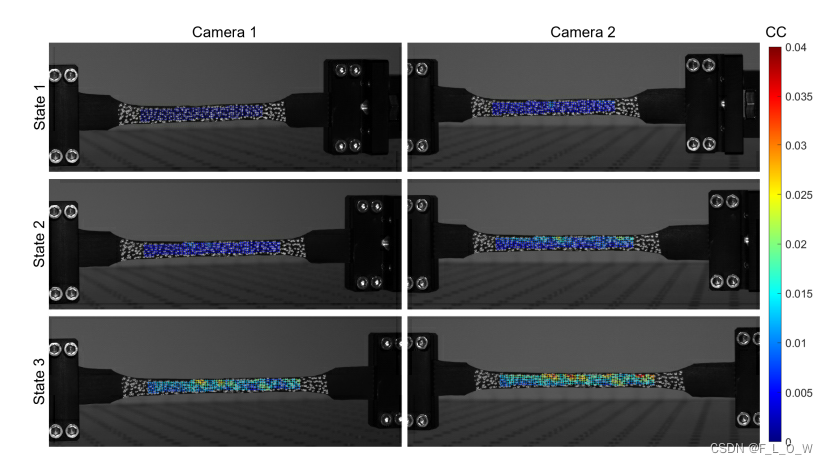
The grid of corresponding matched points are plotted as crosses overlaid on each image, with the colors representing their correlation coefficient (CC) with the reference image (camera 1, state 1, top left panel). 【问： CC为什么这么小？】

Step 3: 3D reconstruction

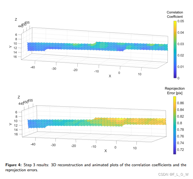
1. The set of matching points on each pair of stereo images are first being undistorted using the intrinsic camera parameters of each camera.
2. Transform the image points into 3D world points using the stereo camera parameters

---

In addition, the reprojection errors are obtained for each point【注意，每一个点的重投影误差都有】, by calculating the distances (in pixels) between the detected and the reprojected points.

Step 4: Post processing

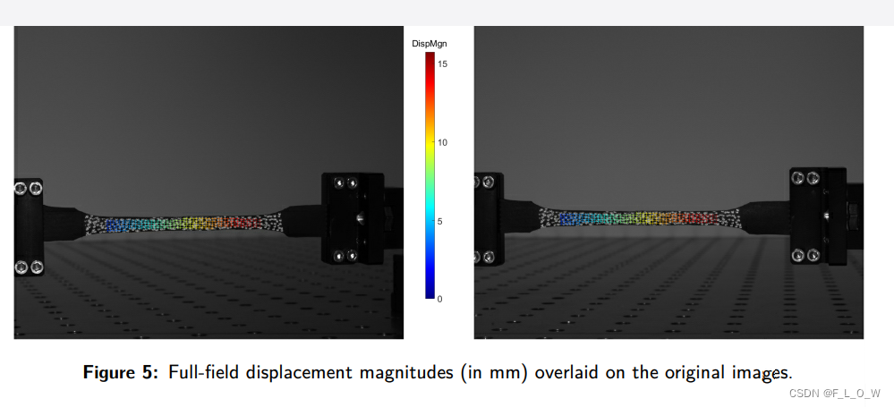
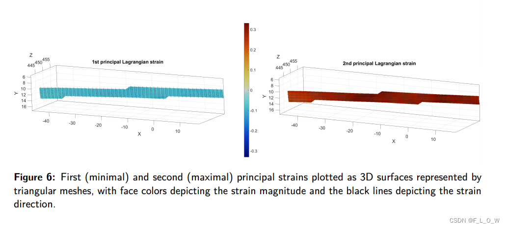
3D coordinates are used to derive the full-field displacement (for each point), deformation (for each triangular element), and strain maps (for each triangular element).

---

For each triangular element, the position vectors of its vertices are used to calculate the deformation gradient tensor $\mathbf{F}$, from which the the right and left Cuchy-Green deformation tensors ( $\mathbf{C}={\mathbf{F}}^{\mathbf{T}}\mathbf{F}$ and $\mathbf{B}=\mathbf{F}{\mathbf{F}}^{\mathbf{T}}$, respectively) are derived, as well as the Green-Lagrangian and Eulerian-Almansi strain tensors ( $\mathbf{E}=0.5(\mathbf{C}-\mathbf{I})$ and $\mathbf{e}=0.5(\mathbf{I}-{\mathbf{B}}^{-1})$.

---

The principal components and directions of these tensors are computed for deriving the principal stretches ${\lambda }_i$ and strains $E_i$ and $e_i$, as well as the equivalent (Von-Mises) strain, maximal shear strain, and the
area change.

Validation using a rigid body motion (RBM) test

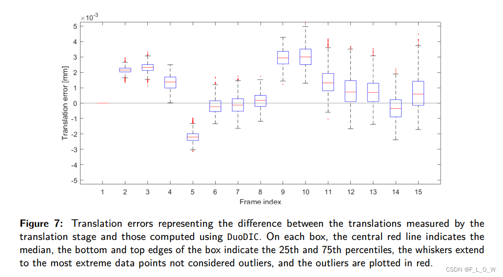
Rigid body motion experiment: a speckled cylinder was translated using a motorized linear translation stage (PT1/M-Z8, Thorlabs, USA), in 15 increments of 0.2mm.

Evaluate: By comparing the displacements measured using the translation stage with those computed using DuoDIC, the displacement errors were quantified, as:

In addition, since strain should vanish for any RBM, any non-zero strains represent measurement errors. Figure 8 plots the strains measured during the RBM translations:

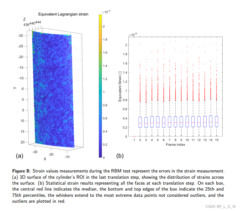
The results indicate that for this experimental setup, the translations were accurate to within $(1.3\pm 1.1).10^{-3}$ mm and the strains errors were $(3.4\pm 2.3).10^{-4}$.

Limitations

1. The number and/or total size of images that can be processed together is limited by Ncorr’s memory limitation;
2. Ncorr’s seed placement process might fail to correctly place the seeds in cases of large deformation. especially if, in addition, the stereo angle between the cameras is large.

遗留问题

1. 为什么2D-DIC中的CC数值这么小？
2. 为什么窗口会开的这么大？【潘兵老师的论文】
3. Cosserat point element method？描述变形？
4. right and left Cuchy-Green deformation tensors ？

参考资料

https://joss.theoj.org/papers/10.21105/joss.04279

附录

1. strain gages: 应变计
2. extensometers： 伸长计
3. proprietary： 专有
4. experimental mechanics: 实验力学
5. The principal components： 主分量
6. metrological performance: 计量性能

• a main advantages of an open-source software is the ability to compare results and performance, and to cross-validate the implementation of different algorithms and approaches.

• For each triangular element, the position vectors of its vertices are used to calculate the deformation gradient tensor $\mathbf{F}$, from which the the right and left Cuchy-Green deformation tensors ( $\mathbf{C}={\mathbf{F}}^{\mathbf{T}}\mathbf{F}$ and $\mathbf{B}=\mathbf{F}{\mathbf{F}}^{\mathbf{T}}$, respectively) are derived, as well as the Green-Lagrangian and Eulerian-Almansi strain tensors ( $\mathbf{E}=0.5(\mathbf{C}-\mathbf{I})$ and $\mathbf{e}=0.5(\mathbf{I}-{\mathbf{B}}^{-1})$. 【from which的语法值得学习】