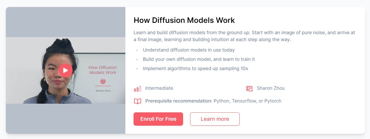
How Diffusion Models Work

本文是 https://www.deeplearning.ai/short-courses/how-diffusion-models-work/ 这门课程的学习笔记。

How Diffusion Models Work：Sharon Zhou

What you’ll learn in this course

In How Diffusion Models Work, you will gain a deep familiarity with the diffusion process and the models which carry it out. More than simply pulling in a pre-built model or using an API, this course will teach you to build a diffusion model from scratch.

In this course you will:

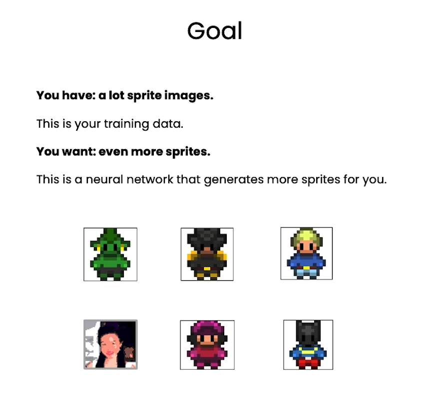
• Explore the cutting-edge world of diffusion-based generative AI and create your own diffusion model from scratch.
• Gain deep familiarity with the diffusion process and the models driving it, going beyond pre-built models and APIs.
• Acquire practical coding skills by working through labs on sampling, training diffusion models, building neural networks for noise prediction, and adding context for personalized image generation.

At the end of the course, you will have a model that can serve as a starting point for your own exploration of diffusion models for your applications.

This one-hour course, taught by Sharon Zhou will expand your generative AI capabilities to include building, training, and optimizing diffusion models.

Hands-on examples make the concepts easy to understand and build upon. Built-in Jupyter notebooks allow you to seamlessly experiment with the code and labs presented in the course.

[1] Intuition

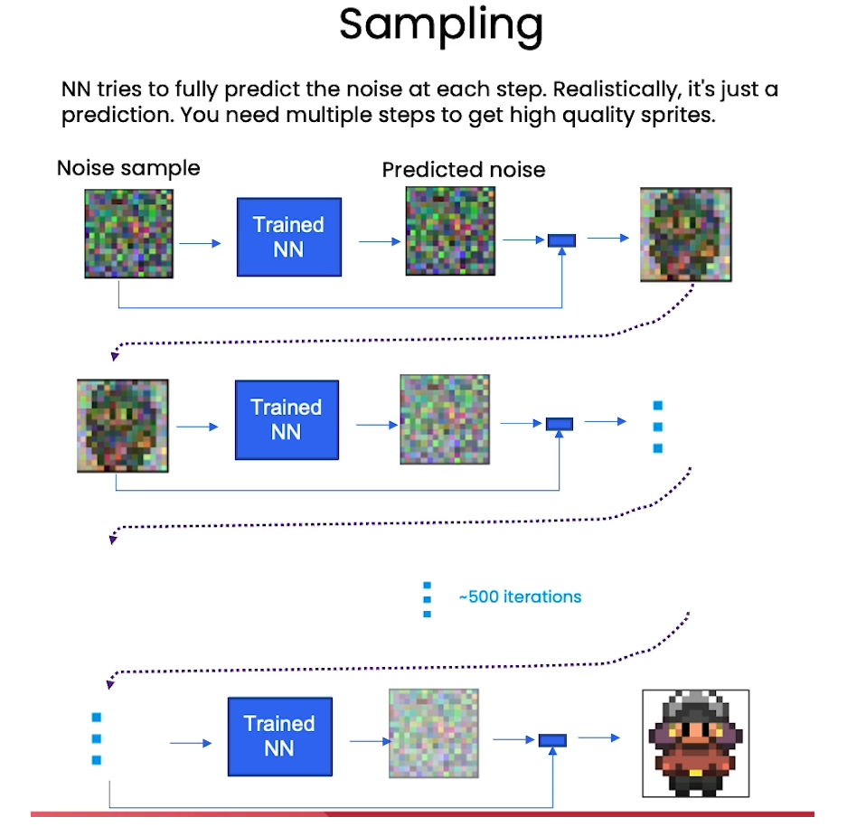
[2] Sampling

from typing import Dict, Tuple
from tqdm import tqdm
import torch
import torch.nn as nn
import torch.nn.functional as F
from torch.utils.data import DataLoader
from torchvision import models, transforms
from torchvision.utils import save_image, make_grid
import matplotlib.pyplot as plt
from matplotlib.animation import FuncAnimation, PillowWriter
import numpy as np
from IPython.display import HTML
from diffusion_utilities import *

Setting Things Up

class ContextUnet(nn.Module):
    def __init__(self, in_channels, n_feat=256, n_cfeat=10, height=28):  # cfeat - context features
        super(ContextUnet, self).__init__()

        # number of input channels, number of intermediate feature maps and number of classes
        self.in_channels = in_channels
        self.n_feat = n_feat
        self.n_cfeat = n_cfeat
        self.h = height  #assume h == w. must be divisible by 4, so 28,24,20,16...

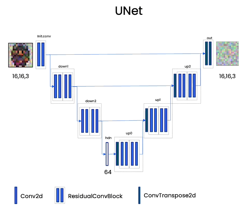
        # Initialize the initial convolutional layer
        self.init_conv = ResidualConvBlock(in_channels, n_feat, is_res=True)

        # Initialize the down-sampling path of the U-Net with two levels
        self.down1 = UnetDown(n_feat, n_feat)        # down1 #[10, 256, 8, 8]
        self.down2 = UnetDown(n_feat, 2 * n_feat)    # down2 #[10, 256, 4,  4]
        
         # original: self.to_vec = nn.Sequential(nn.AvgPool2d(7), nn.GELU())
        self.to_vec = nn.Sequential(nn.AvgPool2d((4)), nn.GELU())

        # Embed the timestep and context labels with a one-layer fully connected neural network
        self.timeembed1 = EmbedFC(1, 2*n_feat)
        self.timeembed2 = EmbedFC(1, 1*n_feat)
        self.contextembed1 = EmbedFC(n_cfeat, 2*n_feat)
        self.contextembed2 = EmbedFC(n_cfeat, 1*n_feat)

        # Initialize the up-sampling path of the U-Net with three levels
        self.up0 = nn.Sequential(
            nn.ConvTranspose2d(2 * n_feat, 2 * n_feat, self.h//4, self.h//4), # up-sample  
            nn.GroupNorm(8, 2 * n_feat), # normalize                       
            nn.ReLU(),
        )
        self.up1 = UnetUp(4 * n_feat, n_feat)
        self.up2 = UnetUp(2 * n_feat, n_feat)

        # Initialize the final convolutional layers to map to the same number of channels as the input image
        self.out = nn.Sequential(
            nn.Conv2d(2 * n_feat, n_feat, 3, 1, 1), # reduce number of feature maps   #in_channels, out_channels, kernel_size, stride=1, padding=0
            nn.GroupNorm(8, n_feat), # normalize
            nn.ReLU(),
            nn.Conv2d(n_feat, self.in_channels, 3, 1, 1), # map to same number of channels as input
        )

    def forward(self, x, t, c=None):
        """
        x : (batch, n_feat, h, w) : input image
        t : (batch, n_cfeat)      : time step
        c : (batch, n_classes)    : context label
        """
        # x is the input image, c is the context label, t is the timestep, context_mask says which samples to block the context on

        # pass the input image through the initial convolutional layer
        x = self.init_conv(x)
        # pass the result through the down-sampling path
        down1 = self.down1(x)       #[10, 256, 8, 8]
        down2 = self.down2(down1)   #[10, 256, 4, 4]
        
        # convert the feature maps to a vector and apply an activation
        hiddenvec = self.to_vec(down2) # hiddenvec 的维度应该为 [10, 256, 1, 1]
        # AvgPool2d((4)) 操作：
		#这个操作是一个平均池化（Average Pooling）层，将特征图的每个 4x4 区域的值取平均。由于特征图 down2 的维度为 [10, 256, 4, 4]，经过 				#AvgPool2d((4)) 操作后，每个特征图将被降采样为一个单一的值。因此，输出的形状将变为 [10, 256, 1, 1]。
        # mask out context if context_mask == 1
        if c is None:
            c = torch.zeros(x.shape[0], self.n_cfeat).to(x)
            
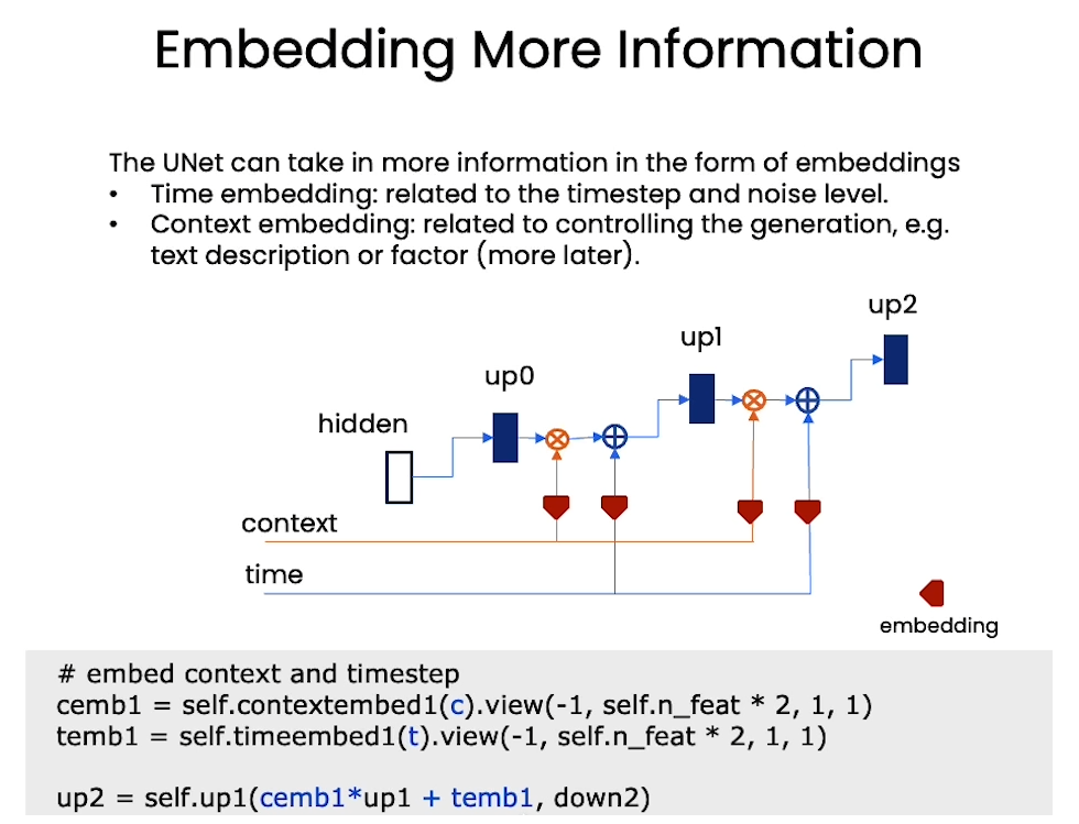
        # embed context and timestep
        cemb1 = self.contextembed1(c).view(-1, self.n_feat * 2, 1, 1)     # (batch, 2*n_feat, 1,1)
        temb1 = self.timeembed1(t).view(-1, self.n_feat * 2, 1, 1)
        cemb2 = self.contextembed2(c).view(-1, self.n_feat, 1, 1)
        temb2 = self.timeembed2(t).view(-1, self.n_feat, 1, 1)
        print(f"uunet forward: cemb1 {cemb1.shape}. temb1 {temb1.shape}, cemb2 {cemb2.shape}. temb2 {temb2.shape}")
        # uunet forward: cemb1 torch.Size([32, 128, 1, 1]). 
        # temb1 torch.Size([1, 128, 1, 1]), 
        # cemb2 torch.Size([32, 64, 1, 1]). 
        # temb2 torch.Size([1, 64, 1, 1])

        up1 = self.up0(hiddenvec) # hiddenvec 的维度应该为 [10, 256, 1, 1]
        up2 = self.up1(cemb1*up1 + temb1, down2)  # add and multiply embeddings
        up3 = self.up2(cemb2*up2 + temb2, down1)
        out = self.out(torch.cat((up3, x), 1))
        return out

根据代码和已知信息，我们可以推断 up1, up2, up3 和 out 的输出维度如下：

1. 对于 up1：

   • 输入是 hiddenvec，其形状为 (batch_size, n_feat, 1, 1)。
   • up0 中的转置卷积操作会将输入进行上采样，输出的形状将与 down2 的特征图相同，即 (batch_size, 2*n_feat, h/4, w/4)。

2. 对于 up2：

   • 输入是 cemb1 * up1 + temb1，其中 cemb1 的形状为 (batch_size, 2*n_feat, 1, 1)，up1 的形状为 (batch_size, 2*n_feat, h/4, w/4)，temb1 的形状为 (batch_size, 2*n_feat, 1, 1)。
   • 这些张量相加后，其形状应该仍然是 (batch_size, 2*n_feat, h/4, w/4)。
   • up1 中的上采样操作将输出的特征图大小恢复为原来的一半，因此，up2 的输出形状将是 (batch_size, n_feat, h/2, w/2)。

3. 对于 up3：

   • 输入是 cemb2 * up2 + temb2，其中 cemb2 的形状为 (batch_size, n_feat, 1, 1)，up2 的形状为 (batch_size, n_feat, h/2, w/2)，temb2 的形状为 (batch_size, n_feat, 1, 1)。
   • 这些张量相加后，其形状应该仍然是 (batch_size, n_feat, h/2, w/2)。
   • up2 中的上采样操作将输出的特征图大小恢复为原来的一半，因此，up3 的输出形状将是 (batch_size, n_feat, h, w)。

4. 对于 out：

   • 输入是将 up3 和原始输入 x 拼接在一起，up3 的形状为 (batch_size, n_feat, h, w)，x 的形状为 (batch_size, in_channels, h, w)。
   • 因此，拼接后输入通道的数量为 n_feat + in_channels。
   • out 的输出形状应该是 (batch_size, in_channels, h, w)，与原始输入的图像大小相同。

综上所述，up1 的输出形状为 (batch_size, 2*n_feat, h/4, w/4)，up2 的输出形状为 (batch_size, n_feat, h/2, w/2)，up3 的输出形状为 (batch_size, n_feat, h, w)，而 out 的输出形状应该是 (batch_size, in_channels, h, w)。

有用的函数：diffusion_utilities.py文件如下

import torch
import torch.nn as nn
import numpy as np
from torchvision.utils import save_image, make_grid
import matplotlib.pyplot as plt
from matplotlib.animation import FuncAnimation, PillowWriter
import os
import torchvision.transforms as transforms
from torch.utils.data import Dataset
from PIL import Image


class ResidualConvBlock(nn.Module):
    def __init__(
        self, in_channels: int, out_channels: int, is_res: bool = False
    ) -> None:
        super().__init__()

        # Check if input and output channels are the same for the residual connection
        self.same_channels = in_channels == out_channels

        # Flag for whether or not to use residual connection
        self.is_res = is_res

        # First convolutional layer
        self.conv1 = nn.Sequential(
            nn.Conv2d(in_channels, out_channels, 3, 1, 1),   # 3x3 kernel with stride 1 and padding 1
            nn.BatchNorm2d(out_channels),   # Batch normalization
            nn.GELU(),   # GELU activation function
        )

        # Second convolutional layer
        self.conv2 = nn.Sequential(
            nn.Conv2d(out_channels, out_channels, 3, 1, 1),   # 3x3 kernel with stride 1 and padding 1
            nn.BatchNorm2d(out_channels),   # Batch normalization
            nn.GELU(),   # GELU activation function
        )

    def forward(self, x: torch.Tensor) -> torch.Tensor:

        # If using residual connection
        if self.is_res:
            # Apply first convolutional layer
            x1 = self.conv1(x)

            # Apply second convolutional layer
            x2 = self.conv2(x1)

            # If input and output channels are the same, add residual connection directly
            if self.same_channels:
                out = x + x2
            else:
                # If not, apply a 1x1 convolutional layer to match dimensions before adding residual connection
                shortcut = nn.Conv2d(x.shape[1], x2.shape[1], kernel_size=1, stride=1, padding=0).to(x.device)
                out = shortcut(x) + x2
            #print(f"resconv forward: x {x.shape}, x1 {x1.shape}, x2 {x2.shape}, out {out.shape}")

            # Normalize output tensor
            return out / 1.414

        # If not using residual connection, return output of second convolutional layer
        else:
            x1 = self.conv1(x)
            x2 = self.conv2(x1)
            return x2

    # Method to get the number of output channels for this block
    def get_out_channels(self):
        return self.conv2[0].out_channels

    # Method to set the number of output channels for this block
    def set_out_channels(self, out_channels):
        self.conv1[0].out_channels = out_channels
        self.conv2[0].in_channels = out_channels
        self.conv2[0].out_channels = out_channels

        

class UnetUp(nn.Module):
    def __init__(self, in_channels, out_channels):
        super(UnetUp, self).__init__()
        
        # Create a list of layers for the upsampling block
        # The block consists of a ConvTranspose2d layer for upsampling, followed by two ResidualConvBlock layers
        layers = [
            nn.ConvTranspose2d(in_channels, out_channels, 2, 2),
            ResidualConvBlock(out_channels, out_channels),
            ResidualConvBlock(out_channels, out_channels),
        ]
        
        # Use the layers to create a sequential model
        self.model = nn.Sequential(*layers)

    def forward(self, x, skip):
        # Concatenate the input tensor x with the skip connection tensor along the channel dimension
        x = torch.cat((x, skip), 1)
        
        # Pass the concatenated tensor through the sequential model and return the output
        x = self.model(x)
        return x

    
class UnetDown(nn.Module):
    def __init__(self, in_channels, out_channels):
        super(UnetDown, self).__init__()
        
        # Create a list of layers for the downsampling block
        # Each block consists of two ResidualConvBlock layers, followed by a MaxPool2d layer for downsampling
        layers = [ResidualConvBlock(in_channels, out_channels), ResidualConvBlock(out_channels, out_channels), nn.MaxPool2d(2)]
        
        # Use the layers to create a sequential model
        self.model = nn.Sequential(*layers)

    def forward(self, x):
        # Pass the input through the sequential model and return the output
        return self.model(x)

class EmbedFC(nn.Module):
    def __init__(self, input_dim, emb_dim):
        super(EmbedFC, self).__init__()
        '''
        This class defines a generic one layer feed-forward neural network for embedding input data of
        dimensionality input_dim to an embedding space of dimensionality emb_dim.
        '''
        self.input_dim = input_dim
        
        # define the layers for the network
        layers = [
            nn.Linear(input_dim, emb_dim),
            nn.GELU(),
            nn.Linear(emb_dim, emb_dim),
        ]
        
        # create a PyTorch sequential model consisting of the defined layers
        self.model = nn.Sequential(*layers)

    def forward(self, x):
        # flatten the input tensor
        x = x.view(-1, self.input_dim)
        # apply the model layers to the flattened tensor
        return self.model(x)
   

测试ResidualConvBlock类

import torch
import torch.nn as nn

# 创建一个ResidualConvBlock实例
residual_block = ResidualConvBlock(in_channels=3, out_channels=3, is_res=True)

# 创建一个测试输入张量
x = torch.randn(1, 3, 32, 32)  # 假设输入张量的形状为(batch_size, in_channels, height, width)

# 使用ResidualConvBlock进行前向传播
output = residual_block(x)

print(output.shape)

这个例子假设输入张量的形状是 (1, 3, 32, 32)，即一个 3 通道、高度和宽度均为 32 像素的图像。在这个例子中，我们使用了残差连接，并且输入和输出通道数量相同。我们预期输出应该与输入张量的形状相同 (1, 3, 32, 32)。

# hyperparameters

# diffusion hyperparameters
timesteps = 500
beta1 = 1e-4
beta2 = 0.02

# network hyperparameters
device = torch.device("cuda:0" if torch.cuda.is_available() else torch.device('cpu'))
n_feat = 64 # 64 hidden dimension feature
n_cfeat = 5 # context vector is of size 5
height = 16 # 16x16 image
save_dir = './weights/'

# construct DDPM noise schedule
b_t = (beta2 - beta1) * torch.linspace(0, 1, timesteps + 1, device=device) + beta1
a_t = 1 - b_t
ab_t = torch.cumsum(a_t.log(), dim=0).exp()    
ab_t[0] = 1

# construct model
nn_model = ContextUnet(in_channels=3, n_feat=n_feat, n_cfeat=n_cfeat, height=height).to(device)

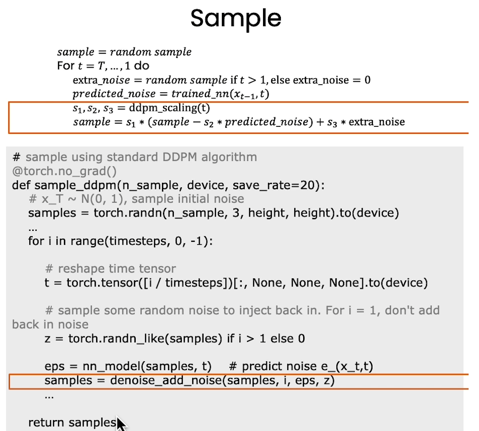
Sampling

# helper function; removes the predicted noise (but adds some noise back in to avoid collapse)
def denoise_add_noise(x, t, pred_noise, z=None):
    if z is None:
        z = torch.randn_like(x)
    noise = b_t.sqrt()[t] * z
    mean = (x - pred_noise * ((1 - a_t[t]) / (1 - ab_t[t]).sqrt())) / a_t[t].sqrt()
    return mean + noise

# load in model weights and set to eval mode
nn_model.load_state_dict(torch.load(f"{save_dir}/model_trained.pth", map_location=device))
nn_model.eval()
print("Loaded in Model")

# sample using standard algorithm
@torch.no_grad()
def sample_ddpm(n_sample, save_rate=20):
    # x_T ~ N(0, 1), sample initial noise
    samples = torch.randn(n_sample, 3, height, height).to(device)  

    # array to keep track of generated steps for plotting
    intermediate = [] 
    for i in range(timesteps, 0, -1):
        print(f'sampling timestep {i:3d}', end='\r')

        # reshape time tensor
        t = torch.tensor([i / timesteps])[:, None, None, None].to(device)

        # sample some random noise to inject back in. For i = 1, don't add back in noise
        z = torch.randn_like(samples) if i > 1 else 0

        eps = nn_model(samples, t)    # predict noise e_(x_t,t)
        samples = denoise_add_noise(samples, i, eps, z)
        if i % save_rate ==0 or i==timesteps or i<8:
            intermediate.append(samples.detach().cpu().numpy())

    intermediate = np.stack(intermediate)
    return samples, intermediate

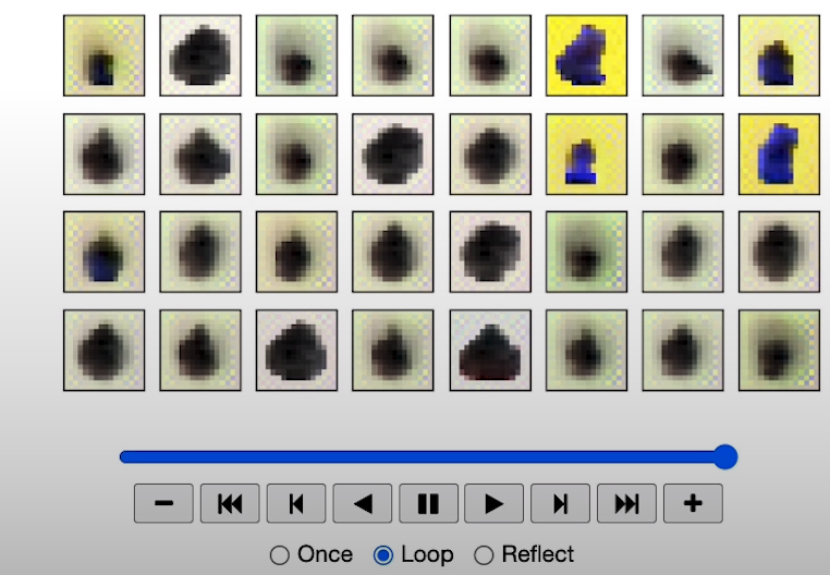
# visualize samples
plt.clf()
samples, intermediate_ddpm = sample_ddpm(32)
animation_ddpm = plot_sample(intermediate_ddpm,32,4,save_dir, "ani_run", None, save=False)
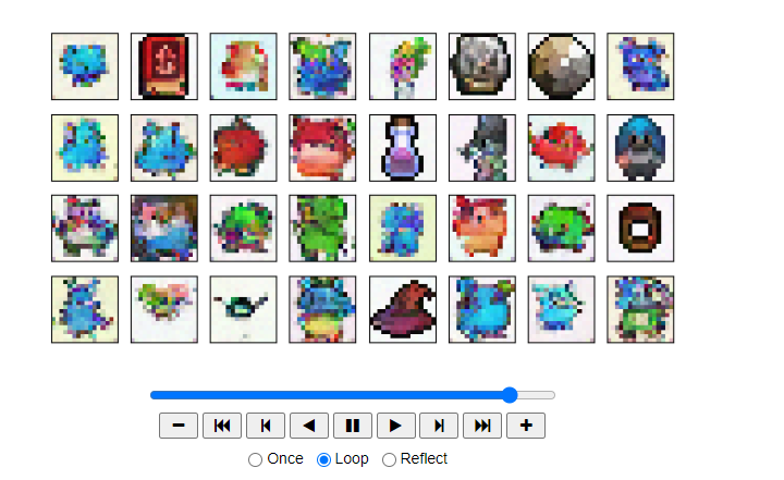
HTML(animation_ddpm.to_jshtml())

Output

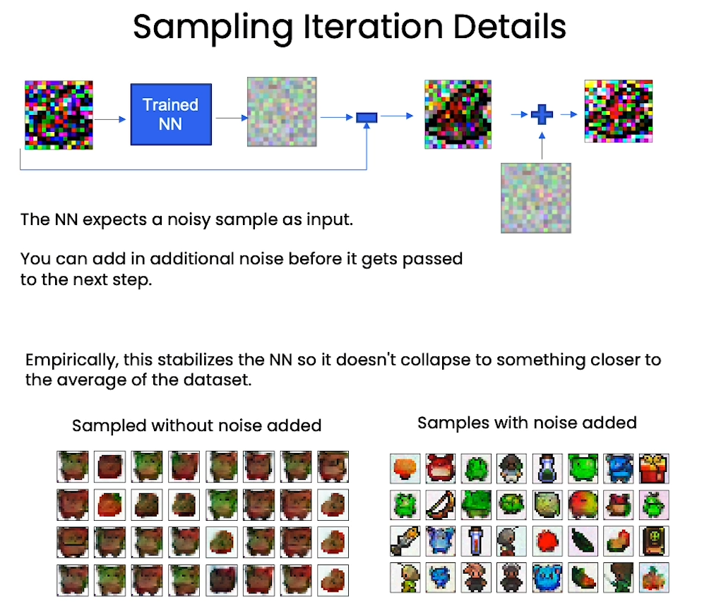
Demonstrate incorrectly sample without adding the ‘extra noise’

# incorrectly sample without adding in noise
@torch.no_grad()
def sample_ddpm_incorrect(n_sample):
    # x_T ~ N(0, 1), sample initial noise
    samples = torch.randn(n_sample, 3, height, height).to(device)  

    # array to keep track of generated steps for plotting
    intermediate = [] 
    for i in range(timesteps, 0, -1):
        print(f'sampling timestep {i:3d}', end='\r')

        # reshape time tensor
        # [:, None, None, None] 是一种广播操作，用于在 PyTorch 中扩展张量的维度。
        # 这段代码的作用是创建一个时间张量 t，该张量的形状为 (1, 1, 1, 1)
        t = torch.tensor([i / timesteps])[:, None, None, None].to(device)

        # don't add back in noise
        z = 0

        eps = nn_model(samples, t)    # predict noise e_(x_t,t)
        samples = denoise_add_noise(samples, i, eps, z)
        if i%20==0 or i==timesteps or i<8:
            intermediate.append(samples.detach().cpu().numpy())

    intermediate = np.stack(intermediate)
    return samples, intermediate

# visualize samples
plt.clf()
samples, intermediate = sample_ddpm_incorrect(32)
animation = plot_sample(intermediate,32,4,save_dir, "ani_run", None, save=False)
HTML(animation.to_jshtml())

Output

Acknowledgments

Sprites by ElvGames, FrootsnVeggies and kyrise
This code is modified from, https://github.com/cloneofsimo/minDiffusion
Diffusion model is based on Denoising Diffusion Probabilistic Models and Denoising Diffusion Implicit Models

[3] Neural Network

[4] Training

from typing import Dict, Tuple
from tqdm import tqdm
import torch
import torch.nn as nn
import torch.nn.functional as F
from torch.utils.data import DataLoader
from torchvision import models, transforms
from torchvision.utils import save_image, make_grid
import matplotlib.pyplot as plt
from matplotlib.animation import FuncAnimation, PillowWriter
import numpy as np
from IPython.display import HTML
from diffusion_utilities import *

Setting Things Up

class ContextUnet(nn.Module):
    def __init__(self, in_channels, n_feat=256, n_cfeat=10, height=28):  # cfeat - context features
        super(ContextUnet, self).__init__()

        # number of input channels, number of intermediate feature maps and number of classes
        self.in_channels = in_channels
        self.n_feat = n_feat
        self.n_cfeat = n_cfeat
        self.h = height  #assume h == w. must be divisible by 4, so 28,24,20,16...

        # Initialize the initial convolutional layer
        self.init_conv = ResidualConvBlock(in_channels, n_feat, is_res=True)

        # Initialize the down-sampling path of the U-Net with two levels
        self.down1 = UnetDown(n_feat, n_feat)        # down1 #[10, 256, 8, 8]
        self.down2 = UnetDown(n_feat, 2 * n_feat)    # down2 #[10, 256, 4,  4]
        
         # original: self.to_vec = nn.Sequential(nn.AvgPool2d(7), nn.GELU())
        self.to_vec = nn.Sequential(nn.AvgPool2d((4)), nn.GELU())

        # Embed the timestep and context labels with a one-layer fully connected neural network
        self.timeembed1 = EmbedFC(1, 2*n_feat)
        self.timeembed2 = EmbedFC(1, 1*n_feat)
        self.contextembed1 = EmbedFC(n_cfeat, 2*n_feat)
        self.contextembed2 = EmbedFC(n_cfeat, 1*n_feat)

        # Initialize the up-sampling path of the U-Net with three levels
        self.up0 = nn.Sequential(
            nn.ConvTranspose2d(2 * n_feat, 2 * n_feat, self.h//4, self.h//4), # up-sample 
            nn.GroupNorm(8, 2 * n_feat), # normalize                        
            nn.ReLU(),
        )
        self.up1 = UnetUp(4 * n_feat, n_feat)
        self.up2 = UnetUp(2 * n_feat, n_feat)

        # Initialize the final convolutional layers to map to the same number of channels as the input image
        self.out = nn.Sequential(
            nn.Conv2d(2 * n_feat, n_feat, 3, 1, 1), # reduce number of feature maps   #in_channels, out_channels, kernel_size, stride=1, padding=0
            nn.GroupNorm(8, n_feat), # normalize
            nn.ReLU(),
            nn.Conv2d(n_feat, self.in_channels, 3, 1, 1), # map to same number of channels as input
        )

    def forward(self, x, t, c=None):
        """
        x : (batch, n_feat, h, w) : input image
        t : (batch, n_cfeat)      : time step
        c : (batch, n_classes)    : context label
        """
        # x is the input image, c is the context label, t is the timestep, context_mask says which samples to block the context on

        # pass the input image through the initial convolutional layer
        x = self.init_conv(x)
        # pass the result through the down-sampling path
        down1 = self.down1(x)       #[10, 256, 8, 8]
        down2 = self.down2(down1)   #[10, 256, 4, 4]
        
        # convert the feature maps to a vector and apply an activation
        hiddenvec = self.to_vec(down2)
        
        # mask out context if context_mask == 1
        if c is None:
            c = torch.zeros(x.shape[0], self.n_cfeat).to(x)
            
        # embed context and timestep
        cemb1 = self.contextembed1(c).view(-1, self.n_feat * 2, 1, 1)     # (batch, 2*n_feat, 1,1)
        temb1 = self.timeembed1(t).view(-1, self.n_feat * 2, 1, 1)
        cemb2 = self.contextembed2(c).view(-1, self.n_feat, 1, 1)
        temb2 = self.timeembed2(t).view(-1, self.n_feat, 1, 1)
        #print(f"uunet forward: cemb1 {cemb1.shape}. temb1 {temb1.shape}, cemb2 {cemb2.shape}. temb2 {temb2.shape}")


        up1 = self.up0(hiddenvec)
        up2 = self.up1(cemb1*up1 + temb1, down2)  # add and multiply embeddings
        up3 = self.up2(cemb2*up2 + temb2, down1)
        out = self.out(torch.cat((up3, x), 1))
        return out

# hyperparameters

# diffusion hyperparameters
timesteps = 500
beta1 = 1e-4
beta2 = 0.02

# network hyperparameters
device = torch.device("cuda:0" if torch.cuda.is_available() else torch.device('cpu'))
n_feat = 64 # 64 hidden dimension feature
n_cfeat = 5 # context vector is of size 5
height = 16 # 16x16 image
save_dir = './weights/'

# training hyperparameters
batch_size = 100
n_epoch = 32
lrate=1e-3

# construct DDPM noise schedule
b_t = (beta2 - beta1) * torch.linspace(0, 1, timesteps + 1, device=device) + beta1
a_t = 1 - b_t
ab_t = torch.cumsum(a_t.log(), dim=0).exp()    
ab_t[0] = 1

# construct model
nn_model = ContextUnet(in_channels=3, n_feat=n_feat, n_cfeat=n_cfeat, height=height).to(device)

Training

# load dataset and construct optimizer
dataset = CustomDataset("./sprites_1788_16x16.npy", "./sprite_labels_nc_1788_16x16.npy", transform, null_context=False)
dataloader = DataLoader(dataset, batch_size=batch_size, shuffle=True, num_workers=1)
optim = torch.optim.Adam(nn_model.parameters(), lr=lrate)

Output

sprite shape: (89400, 16, 16, 3)
labels shape: (89400, 5)

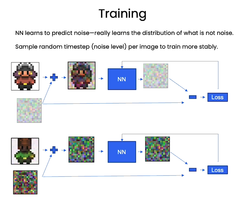
# helper function: perturbs an image to a specified noise level
def perturb_input(x, t, noise):
    return ab_t.sqrt()[t, None, None, None] * x + (1 - ab_t[t, None, None, None]) * noise

This code will take hours to run on a CPU. We recommend you skip this step here and check the intermediate results below.

If you decide to try it, you could download to your own machine. Be sure to change the cell type.
Note, the CPU run time in the course is limited so you will not be able to fully train the network using the class platform.

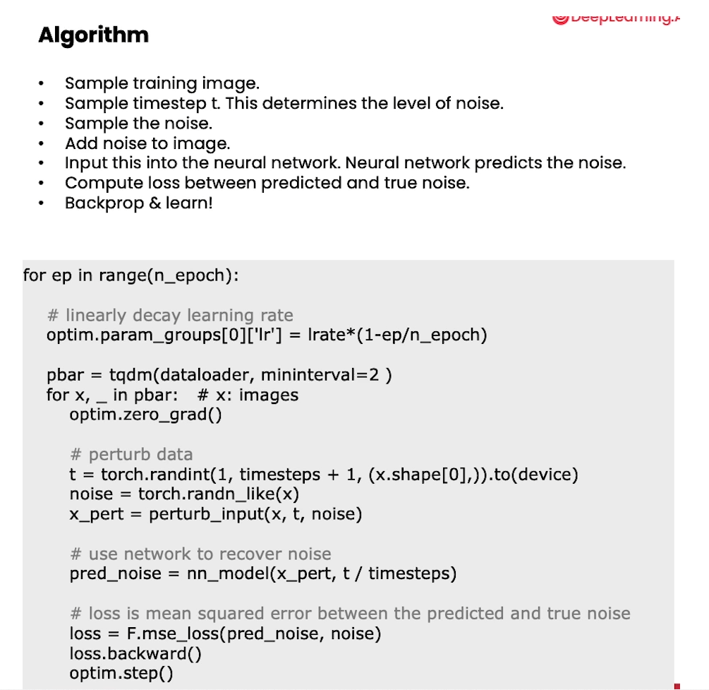
# training without context code

# set into train mode
nn_model.train()

for ep in range(n_epoch):
    print(f'epoch {ep}')
    
    # linearly decay learning rate
    optim.param_groups[0]['lr'] = lrate*(1-ep/n_epoch)
    
    pbar = tqdm(dataloader, mininterval=2 )
    for x, _ in pbar:   # x: images
        optim.zero_grad()
        x = x.to(device)
        
        # perturb data
        noise = torch.randn_like(x)
        t = torch.randint(1, timesteps + 1, (x.shape[0],)).to(device) 
        x_pert = perturb_input(x, t, noise)
        
        # use network to recover noise
        pred_noise = nn_model(x_pert, t / timesteps)
        
        # loss is mean squared error between the predicted and true noise
        loss = F.mse_loss(pred_noise, noise)
        loss.backward()
        
        optim.step()

    # save model periodically
    if ep%4==0 or ep == int(n_epoch-1):
        if not os.path.exists(save_dir):
            os.mkdir(save_dir)
        torch.save(nn_model.state_dict(), save_dir + f"model_{ep}.pth")
        print('saved model at ' + save_dir + f"model_{ep}.pth")

Sampling

# helper function; removes the predicted noise (but adds some noise back in to avoid collapse)
def denoise_add_noise(x, t, pred_noise, z=None):
    if z is None:
        z = torch.randn_like(x)
    noise = b_t.sqrt()[t] * z
    mean = (x - pred_noise * ((1 - a_t[t]) / (1 - ab_t[t]).sqrt())) / a_t[t].sqrt()
    return mean + noise

# sample using standard algorithm
@torch.no_grad()
def sample_ddpm(n_sample, save_rate=20):
    # x_T ~ N(0, 1), sample initial noise
    samples = torch.randn(n_sample, 3, height, height).to(device)  

    # array to keep track of generated steps for plotting
    intermediate = [] 
    for i in range(timesteps, 0, -1):
        print(f'sampling timestep {i:3d}', end='\r')

        # reshape time tensor
        t = torch.tensor([i / timesteps])[:, None, None, None].to(device)

        # sample some random noise to inject back in. For i = 1, don't add back in noise
        z = torch.randn_like(samples) if i > 1 else 0

        eps = nn_model(samples, t)    # predict noise e_(x_t,t)
        samples = denoise_add_noise(samples, i, eps, z)
        if i % save_rate ==0 or i==timesteps or i<8:
            intermediate.append(samples.detach().cpu().numpy())

    intermediate = np.stack(intermediate)
    return samples, intermediate

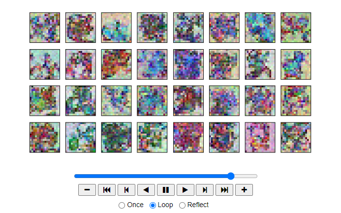
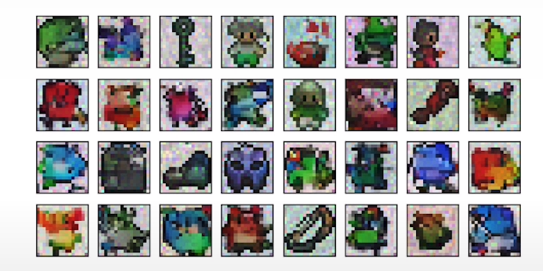
View Epoch 0

# load in model weights and set to eval mode
nn_model.load_state_dict(torch.load(f"{save_dir}/model_0.pth", map_location=device))
nn_model.eval()
print("Loaded in Model")

# visualize samples
plt.clf()
samples, intermediate_ddpm = sample_ddpm(32)
animation_ddpm = plot_sample(intermediate_ddpm,32,4,save_dir, "ani_run", None, save=False)
HTML(animation_ddpm.to_jshtml())

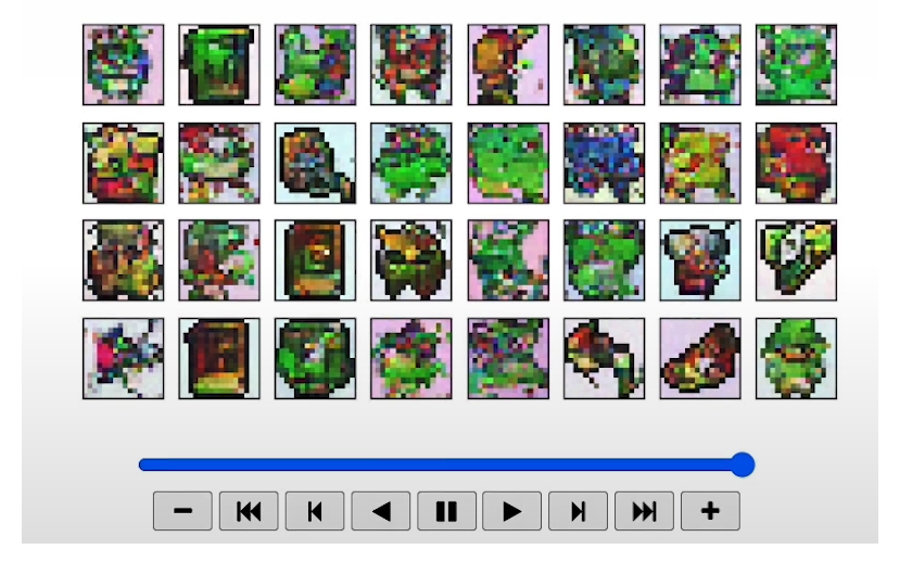
Output

View Epoch 4

# load in model weights and set to eval mode
nn_model.load_state_dict(torch.load(f"{save_dir}/model_4.pth", map_location=device))
nn_model.eval()
print("Loaded in Model")

# visualize samples
plt.clf()
samples, intermediate_ddpm = sample_ddpm(32)
animation_ddpm = plot_sample(intermediate_ddpm,32,4,save_dir, "ani_run", None, save=False)
HTML(animation_ddpm.to_jshtml())

Output

View Epoch 8

# load in model weights and set to eval mode
nn_model.load_state_dict(torch.load(f"{save_dir}/model_8.pth", map_location=device))
nn_model.eval()
print("Loaded in Model")

# visualize samples
plt.clf()
samples, intermediate_ddpm = sample_ddpm(32)
animation_ddpm = plot_sample(intermediate_ddpm,32,4,save_dir, "ani_run", None, save=False)
HTML(animation_ddpm.to_jshtml())

Output

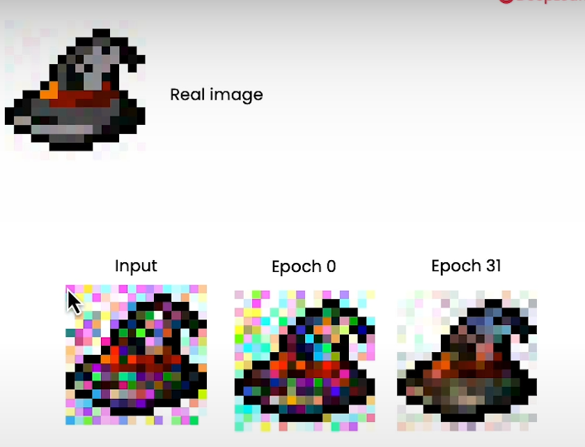
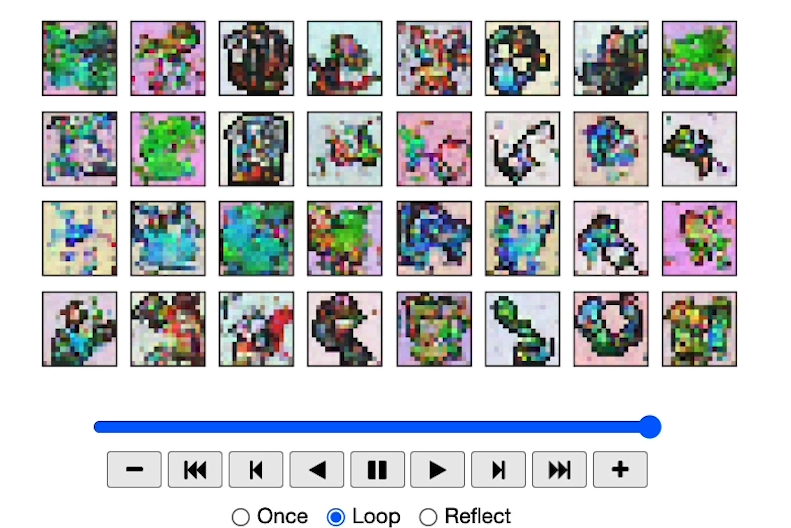
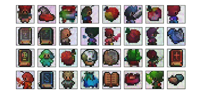
View Epoch 31

# load in model weights and set to eval mode
nn_model.load_state_dict(torch.load(f"{save_dir}/model_31.pth", map_location=device))
nn_model.eval()
print("Loaded in Model")

# visualize samples
plt.clf()
samples, intermediate_ddpm = sample_ddpm(32)
animation_ddpm = plot_sample(intermediate_ddpm,32,4,save_dir, "ani_run", None, save=False)
HTML(animation_ddpm.to_jshtml())

Output

[5] Controlling

from typing import Dict, Tuple
from tqdm import tqdm
import torch
import torch.nn as nn
import torch.nn.functional as F
from torch.utils.data import DataLoader
from torchvision import models, transforms
from torchvision.utils import save_image, make_grid
import matplotlib.pyplot as plt
from matplotlib.animation import FuncAnimation, PillowWriter
import numpy as np
from IPython.display import HTML
from diffusion_utilities import *

Setting Things Up

class ContextUnet(nn.Module):
    def __init__(self, in_channels, n_feat=256, n_cfeat=10, height=28):  # cfeat - context features
        super(ContextUnet, self).__init__()

        # number of input channels, number of intermediate feature maps and number of classes
        self.in_channels = in_channels
        self.n_feat = n_feat
        self.n_cfeat = n_cfeat
        self.h = height  #assume h == w. must be divisible by 4, so 28,24,20,16...

        # Initialize the initial convolutional layer
        self.init_conv = ResidualConvBlock(in_channels, n_feat, is_res=True)

        # Initialize the down-sampling path of the U-Net with two levels
        self.down1 = UnetDown(n_feat, n_feat)        # down1 #[10, 256, 8, 8]
        self.down2 = UnetDown(n_feat, 2 * n_feat)    # down2 #[10, 256, 4,  4]
        
         # original: self.to_vec = nn.Sequential(nn.AvgPool2d(7), nn.GELU())
        self.to_vec = nn.Sequential(nn.AvgPool2d((4)), nn.GELU())

        # Embed the timestep and context labels with a one-layer fully connected neural network
        self.timeembed1 = EmbedFC(1, 2*n_feat)
        self.timeembed2 = EmbedFC(1, 1*n_feat)
        self.contextembed1 = EmbedFC(n_cfeat, 2*n_feat)
        self.contextembed2 = EmbedFC(n_cfeat, 1*n_feat)

        # Initialize the up-sampling path of the U-Net with three levels
        self.up0 = nn.Sequential(
            nn.ConvTranspose2d(2 * n_feat, 2 * n_feat, self.h//4, self.h//4), # up-sample  
            nn.GroupNorm(8, 2 * n_feat), # normalize                        
            nn.ReLU(),
        )
        self.up1 = UnetUp(4 * n_feat, n_feat)
        self.up2 = UnetUp(2 * n_feat, n_feat)

        # Initialize the final convolutional layers to map to the same number of channels as the input image
        self.out = nn.Sequential(
            nn.Conv2d(2 * n_feat, n_feat, 3, 1, 1), # reduce number of feature maps   #in_channels, out_channels, kernel_size, stride=1, padding=0
            nn.GroupNorm(8, n_feat), # normalize
            nn.ReLU(),
            nn.Conv2d(n_feat, self.in_channels, 3, 1, 1), # map to same number of channels as input
        )

    def forward(self, x, t, c=None):
        """
        x : (batch, n_feat, h, w) : input image
        t : (batch, n_cfeat)      : time step
        c : (batch, n_classes)    : context label
        """
        # x is the input image, c is the context label, t is the timestep, context_mask says which samples to block the context on

        # pass the input image through the initial convolutional layer
        x = self.init_conv(x)
        # pass the result through the down-sampling path
        down1 = self.down1(x)       #[10, 256, 8, 8]
        down2 = self.down2(down1)   #[10, 256, 4, 4]
        
        # convert the feature maps to a vector and apply an activation
        hiddenvec = self.to_vec(down2)
        
        # mask out context if context_mask == 1
        if c is None:
            c = torch.zeros(x.shape[0], self.n_cfeat).to(x)
            
        # embed context and timestep
        cemb1 = self.contextembed1(c).view(-1, self.n_feat * 2, 1, 1)     # (batch, 2*n_feat, 1,1)
        temb1 = self.timeembed1(t).view(-1, self.n_feat * 2, 1, 1)
        cemb2 = self.contextembed2(c).view(-1, self.n_feat, 1, 1)
        temb2 = self.timeembed2(t).view(-1, self.n_feat, 1, 1)
        #print(f"uunet forward: cemb1 {cemb1.shape}. temb1 {temb1.shape}, cemb2 {cemb2.shape}. temb2 {temb2.shape}")


        up1 = self.up0(hiddenvec)
        up2 = self.up1(cemb1*up1 + temb1, down2)  # add and multiply embeddings
        up3 = self.up2(cemb2*up2 + temb2, down1)
        out = self.out(torch.cat((up3, x), 1))
        return out

# hyperparameters

# diffusion hyperparameters
timesteps = 500
beta1 = 1e-4
beta2 = 0.02

# network hyperparameters
device = torch.device("cuda:0" if torch.cuda.is_available() else torch.device('cpu'))
n_feat = 64 # 64 hidden dimension feature
n_cfeat = 5 # context vector is of size 5
height = 16 # 16x16 image
save_dir = './weights/'

# training hyperparameters
batch_size = 100
n_epoch = 32
lrate=1e-3

# construct DDPM noise schedule
b_t = (beta2 - beta1) * torch.linspace(0, 1, timesteps + 1, device=device) + beta1
a_t = 1 - b_t
ab_t = torch.cumsum(a_t.log(), dim=0).exp()    
ab_t[0] = 1

# construct model
nn_model = ContextUnet(in_channels=3, n_feat=n_feat, n_cfeat=n_cfeat, height=height).to(device)

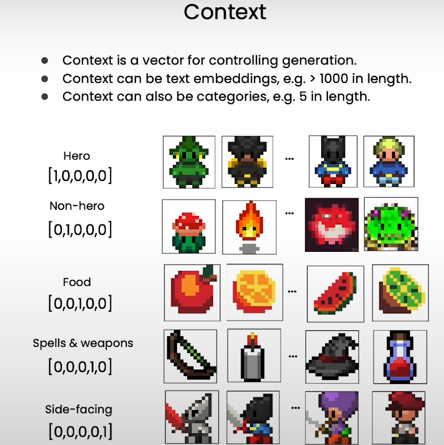
Context

# reset neural network
nn_model = ContextUnet(in_channels=3, n_feat=n_feat, n_cfeat=n_cfeat, height=height).to(device)

# re setup optimizer
optim = torch.optim.Adam(nn_model.parameters(), lr=lrate)

# training with context code
# set into train mode
nn_model.train()

for ep in range(n_epoch):
    print(f'epoch {ep}')
    
    # linearly decay learning rate
    optim.param_groups[0]['lr'] = lrate*(1-ep/n_epoch)
    
    pbar = tqdm(dataloader, mininterval=2 )
    for x, c in pbar:   # x: images  c: context
        optim.zero_grad()
        x = x.to(device)
        c = c.to(x)
        
        # randomly mask out c
        context_mask = torch.bernoulli(torch.zeros(c.shape[0]) + 0.9).to(device)
        c = c * context_mask.unsqueeze(-1)
        
        # perturb data
        noise = torch.randn_like(x)
        t = torch.randint(1, timesteps + 1, (x.shape[0],)).to(device) 
        x_pert = perturb_input(x, t, noise)
        
        # use network to recover noise
        pred_noise = nn_model(x_pert, t / timesteps, c=c)
        
        # loss is mean squared error between the predicted and true noise
        loss = F.mse_loss(pred_noise, noise)
        loss.backward()
        
        optim.step()

    # save model periodically
    if ep%4==0 or ep == int(n_epoch-1):
        if not os.path.exists(save_dir):
            os.mkdir(save_dir)
        torch.save(nn_model.state_dict(), save_dir + f"context_model_{ep}.pth")
        print('saved model at ' + save_dir + f"context_model_{ep}.pth")

# load in pretrain model weights and set to eval mode
nn_model.load_state_dict(torch.load(f"{save_dir}/context_model_trained.pth", map_location=device))
nn_model.eval() 
print("Loaded in Context Model")

Sampling with context

# helper function; removes the predicted noise (but adds some noise back in to avoid collapse)
def denoise_add_noise(x, t, pred_noise, z=None):
    if z is None:
        z = torch.randn_like(x)
    noise = b_t.sqrt()[t] * z
    mean = (x - pred_noise * ((1 - a_t[t]) / (1 - ab_t[t]).sqrt())) / a_t[t].sqrt()
    return mean + noise

# sample with context using standard algorithm
@torch.no_grad()
def sample_ddpm_context(n_sample, context, save_rate=20):
    # x_T ~ N(0, 1), sample initial noise
    samples = torch.randn(n_sample, 3, height, height).to(device)  

    # array to keep track of generated steps for plotting
    intermediate = [] 
    for i in range(timesteps, 0, -1):
        print(f'sampling timestep {i:3d}', end='\r')

        # reshape time tensor
        t = torch.tensor([i / timesteps])[:, None, None, None].to(device)

        # sample some random noise to inject back in. For i = 1, don't add back in noise
        z = torch.randn_like(samples) if i > 1 else 0

        eps = nn_model(samples, t, c=context)    # predict noise e_(x_t,t, ctx)
        samples = denoise_add_noise(samples, i, eps, z)
        if i % save_rate==0 or i==timesteps or i<8:
            intermediate.append(samples.detach().cpu().numpy())

    intermediate = np.stack(intermediate)
    return samples, intermediate

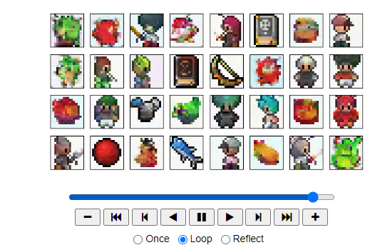
# visualize samples with randomly selected context
plt.clf()
ctx = F.one_hot(torch.randint(0, 5, (32,)), 5).to(device=device).float()
samples, intermediate = sample_ddpm_context(32, ctx)
animation_ddpm_context = plot_sample(intermediate,32,4,save_dir, "ani_run", None, save=False)
HTML(animation_ddpm_context.to_jshtml())

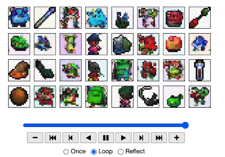
Output

def show_images(imgs, nrow=2):
    _, axs = plt.subplots(nrow, imgs.shape[0] // nrow, figsize=(4,2 ))
    axs = axs.flatten()
    for img, ax in zip(imgs, axs):
        img = (img.permute(1, 2, 0).clip(-1, 1).detach().cpu().numpy() + 1) / 2
        ax.set_xticks([])
        ax.set_yticks([])
        ax.imshow(img)
    plt.show()

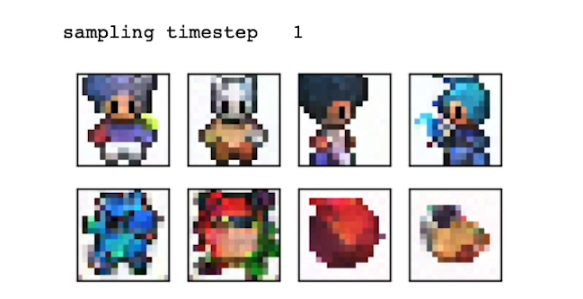
# user defined context
ctx = torch.tensor([
    # hero, non-hero, food, spell, side-facing
    [1,0,0,0,0],  
    [1,0,0,0,0],    
    [0,0,0,0,1],
    [0,0,0,0,1],    
    [0,1,0,0,0],
    [0,1,0,0,0],
    [0,0,1,0,0],
    [0,0,1,0,0],
]).float().to(device)
samples, _ = sample_ddpm_context(ctx.shape[0], ctx)
show_images(samples)

Output

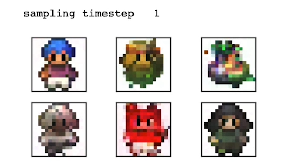
# mix of defined context
ctx = torch.tensor([
    # hero, non-hero, food, spell, side-facing
    [1,0,0,0,0],      #human
    [1,0,0.6,0,0],    
    [0,0,0.6,0.4,0],  
    [1,0,0,0,1],  
    [1,1,0,0,0],
    [1,0,0,1,0]
]).float().to(device)
samples, _ = sample_ddpm_context(ctx.shape[0], ctx)
show_images(samples)

Output

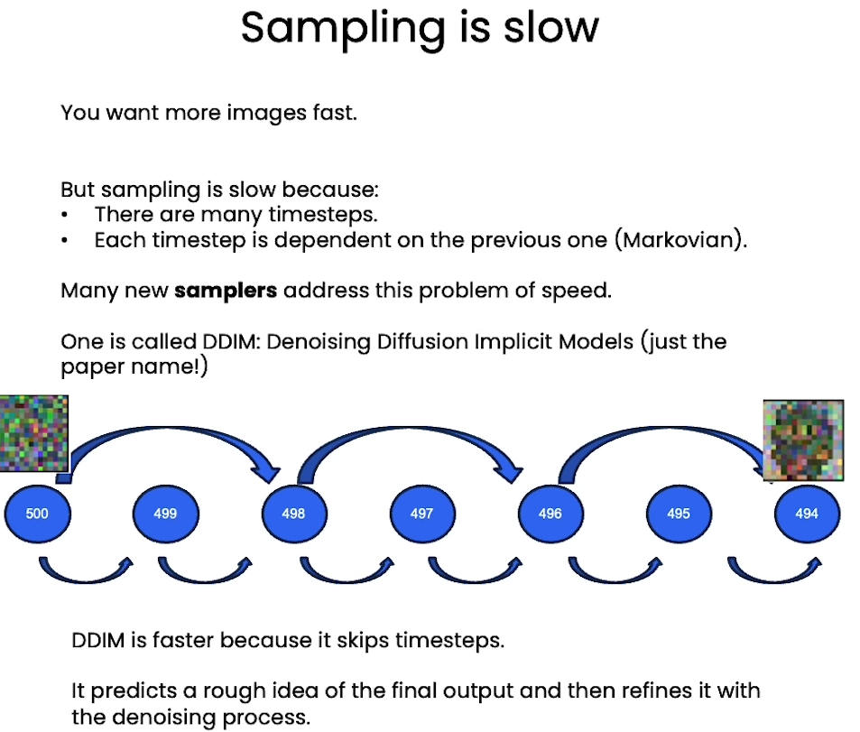
[6] Speeding up

DDIM

DDIM: Denoising Diffusion Implicit Models

from typing import Dict, Tuple
from tqdm import tqdm
import torch
import torch.nn as nn
import torch.nn.functional as F
from torch.utils.data import DataLoader
from torchvision import models, transforms
from torchvision.utils import save_image, make_grid
import matplotlib.pyplot as plt
from matplotlib.animation import FuncAnimation, PillowWriter
import numpy as np
from IPython.display import HTML
from diffusion_utilities import *

Setting Things Up

class ContextUnet(nn.Module):
    def __init__(self, in_channels, n_feat=256, n_cfeat=10, height=28):  # cfeat - context features
        super(ContextUnet, self).__init__()

        # number of input channels, number of intermediate feature maps and number of classes
        self.in_channels = in_channels
        self.n_feat = n_feat
        self.n_cfeat = n_cfeat
        self.h = height  #assume h == w. must be divisible by 4, so 28,24,20,16...

        # Initialize the initial convolutional layer
        self.init_conv = ResidualConvBlock(in_channels, n_feat, is_res=True)

        # Initialize the down-sampling path of the U-Net with two levels
        self.down1 = UnetDown(n_feat, n_feat)        # down1 #[10, 256, 8, 8]
        self.down2 = UnetDown(n_feat, 2 * n_feat)    # down2 #[10, 256, 4,  4]
        
         # original: self.to_vec = nn.Sequential(nn.AvgPool2d(7), nn.GELU())
        self.to_vec = nn.Sequential(nn.AvgPool2d((4)), nn.GELU())

        # Embed the timestep and context labels with a one-layer fully connected neural network
        self.timeembed1 = EmbedFC(1, 2*n_feat)
        self.timeembed2 = EmbedFC(1, 1*n_feat)
        self.contextembed1 = EmbedFC(n_cfeat, 2*n_feat)
        self.contextembed2 = EmbedFC(n_cfeat, 1*n_feat)

        # Initialize the up-sampling path of the U-Net with three levels
        self.up0 = nn.Sequential(
            nn.ConvTranspose2d(2 * n_feat, 2 * n_feat, self.h//4, self.h//4), 
            nn.GroupNorm(8, 2 * n_feat), # normalize                       
            nn.ReLU(),
        )
        self.up1 = UnetUp(4 * n_feat, n_feat)
        self.up2 = UnetUp(2 * n_feat, n_feat)

        # Initialize the final convolutional layers to map to the same number of channels as the input image
        self.out = nn.Sequential(
            nn.Conv2d(2 * n_feat, n_feat, 3, 1, 1), # reduce number of feature maps   #in_channels, out_channels, kernel_size, stride=1, padding=0
            nn.GroupNorm(8, n_feat), # normalize
            nn.ReLU(),
            nn.Conv2d(n_feat, self.in_channels, 3, 1, 1), # map to same number of channels as input
        )

    def forward(self, x, t, c=None):
        """
        x : (batch, n_feat, h, w) : input image
        t : (batch, n_cfeat)      : time step
        c : (batch, n_classes)    : context label
        """
        # x is the input image, c is the context label, t is the timestep, context_mask says which samples to block the context on

        # pass the input image through the initial convolutional layer
        x = self.init_conv(x)
        # pass the result through the down-sampling path
        down1 = self.down1(x)       #[10, 256, 8, 8]
        down2 = self.down2(down1)   #[10, 256, 4, 4]
        
        # convert the feature maps to a vector and apply an activation
        hiddenvec = self.to_vec(down2)
        
        # mask out context if context_mask == 1
        if c is None:
            c = torch.zeros(x.shape[0], self.n_cfeat).to(x)
            
        # embed context and timestep
        cemb1 = self.contextembed1(c).view(-1, self.n_feat * 2, 1, 1)     # (batch, 2*n_feat, 1,1)
        temb1 = self.timeembed1(t).view(-1, self.n_feat * 2, 1, 1)
        cemb2 = self.contextembed2(c).view(-1, self.n_feat, 1, 1)
        temb2 = self.timeembed2(t).view(-1, self.n_feat, 1, 1)
        #print(f"uunet forward: cemb1 {cemb1.shape}. temb1 {temb1.shape}, cemb2 {cemb2.shape}. temb2 {temb2.shape}")


        up1 = self.up0(hiddenvec)
        up2 = self.up1(cemb1*up1 + temb1, down2)  # add and multiply embeddings
        up3 = self.up2(cemb2*up2 + temb2, down1)
        out = self.out(torch.cat((up3, x), 1))
        return out

# hyperparameters

# diffusion hyperparameters
timesteps = 500
beta1 = 1e-4
beta2 = 0.02

# network hyperparameters
device = torch.device("cuda:0" if torch.cuda.is_available() else torch.device('cpu'))
n_feat = 64 # 64 hidden dimension feature
n_cfeat = 5 # context vector is of size 5
height = 16 # 16x16 image
save_dir = './weights/'

# training hyperparameters
batch_size = 100
n_epoch = 32
lrate=1e-3

# construct DDPM noise schedule
b_t = (beta2 - beta1) * torch.linspace(0, 1, timesteps + 1, device=device) + beta1
a_t = 1 - b_t
ab_t = torch.cumsum(a_t.log(), dim=0).exp()    
ab_t[0] = 1

# construct model
nn_model = ContextUnet(in_channels=3, n_feat=n_feat, n_cfeat=n_cfeat, height=height).to(device)

Fast Sampling

# define sampling function for DDIM   
# removes the noise using ddim
def denoise_ddim(x, t, t_prev, pred_noise):
    ab = ab_t[t]
    ab_prev = ab_t[t_prev]
    
    x0_pred = ab_prev.sqrt() / ab.sqrt() * (x - (1 - ab).sqrt() * pred_noise)
    dir_xt = (1 - ab_prev).sqrt() * pred_noise

    return x0_pred + dir_xt

# load in model weights and set to eval mode
nn_model.load_state_dict(torch.load(f"{save_dir}/model_31.pth", map_location=device))
nn_model.eval() 
print("Loaded in Model without context")

# sample quickly using DDIM
@torch.no_grad()
def sample_ddim(n_sample, n=20):
    # x_T ~ N(0, 1), sample initial noise
    samples = torch.randn(n_sample, 3, height, height).to(device)  

    # array to keep track of generated steps for plotting
    intermediate = [] 
    step_size = timesteps // n
    for i in range(timesteps, 0, -step_size):
        print(f'sampling timestep {i:3d}', end='\r')

        # reshape time tensor
        t = torch.tensor([i / timesteps])[:, None, None, None].to(device)

        eps = nn_model(samples, t)    # predict noise e_(x_t,t)
        samples = denoise_ddim(samples, i, i - step_size, eps)
        intermediate.append(samples.detach().cpu().numpy())

    intermediate = np.stack(intermediate)
    return samples, intermediate

# visualize samples
plt.clf()
samples, intermediate = sample_ddim(32, n=25)
animation_ddim = plot_sample(intermediate,32,4,save_dir, "ani_run", None, save=False)
HTML(animation_ddim.to_jshtml())

Output

# load in model weights and set to eval mode
nn_model.load_state_dict(torch.load(f"{save_dir}/context_model_31.pth", map_location=device))
nn_model.eval() 
print("Loaded in Context Model")

# fast sampling algorithm with context
@torch.no_grad()
def sample_ddim_context(n_sample, context, n=20):
    # x_T ~ N(0, 1), sample initial noise
    samples = torch.randn(n_sample, 3, height, height).to(device)  

    # array to keep track of generated steps for plotting
    intermediate = [] 
    step_size = timesteps // n
    for i in range(timesteps, 0, -step_size):
        print(f'sampling timestep {i:3d}', end='\r')

        # reshape time tensor
        t = torch.tensor([i / timesteps])[:, None, None, None].to(device)

        eps = nn_model(samples, t, c=context)    # predict noise e_(x_t,t)
        samples = denoise_ddim(samples, i, i - step_size, eps)
        intermediate.append(samples.detach().cpu().numpy())

    intermediate = np.stack(intermediate)
    return samples, intermediate

# visualize samples
plt.clf()
ctx = F.one_hot(torch.randint(0, 5, (32,)), 5).to(device=device).float()
samples, intermediate = sample_ddim_context(32, ctx)
animation_ddpm_context = plot_sample(intermediate,32,4,save_dir, "ani_run", None, save=False)
HTML(animation_ddpm_context.to_jshtml())

Output

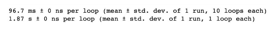
Compare DDPM, DDIM speed

# helper function; removes the predicted noise (but adds some noise back in to avoid collapse)
def denoise_add_noise(x, t, pred_noise, z=None):
    if z is None:
        z = torch.randn_like(x)
    noise = b_t.sqrt()[t] * z
    mean = (x - pred_noise * ((1 - a_t[t]) / (1 - ab_t[t]).sqrt())) / a_t[t].sqrt()
    return mean + noise

# sample using standard algorithm
@torch.no_grad()
def sample_ddpm(n_sample, save_rate=20):
    # x_T ~ N(0, 1), sample initial noise
    samples = torch.randn(n_sample, 3, height, height).to(device)  

    # array to keep track of generated steps for plotting
    intermediate = [] 
    for i in range(timesteps, 0, -1):
        print(f'sampling timestep {i:3d}', end='\r')

        # reshape time tensor
        t = torch.tensor([i / timesteps])[:, None, None, None].to(device)

        # sample some random noise to inject back in. For i = 1, don't add back in noise
        z = torch.randn_like(samples) if i > 1 else 0

        eps = nn_model(samples, t)    # predict noise e_(x_t,t)
        samples = denoise_add_noise(samples, i, eps, z)
        if i % save_rate ==0 or i==timesteps or i<8:
            intermediate.append(samples.detach().cpu().numpy())

    intermediate = np.stack(intermediate)
    return samples, intermediate

%timeit -r 1 sample_ddim(32, n=25)
%timeit -r 1 sample_ddpm(32, )

Output

后记

经过2天的时间，大概2小时，完成这门课的学习。代码是给定的，所以没有自己写代码的过程，但是让我对扩散模型有了一定的了解，想要更深入的理解扩散模型，还是需要阅读论文和相关资料。这门课仅仅是入门课。