物以类聚人以群分。
什么是聚类呢?

1、核心思想和原理
聚类的目的
同簇高相似度
不同簇高相异度
同类尽量相聚
不同类尽量分离
聚类和分类的区别
分类 classification
监督学习
训练获得分类器
预测未知数据
聚类 clustering
无监督学习,不关心类别标签
没有训练过程
算法自己要根据定义的规则将相似的样本划分到一起,不相似的样本分成不同的类别,不同的簇
簇 Cluster
簇内样本之间的距离,或样本点在数据空间的密度
对簇的不同定义可以得到不同的算法

主要聚类方法

聚类步骤
- 数据准备:特征的标准化和降维
- 特征选择:最有效特征,并将其存储在向量当中
- 特征提取:特征转换,通过对选择的特征进行一些转换,形成更突出的特征
- 聚类:基于某种距离做相似度度量,得到簇
- 结果评估:分析聚类结果
2、K-means和分层聚类
2.1、基于划分的聚类方式
将对象划分为互斥的簇
每个对象仅属于一个簇
簇间相似性低,簇内相似性高
K-均值分类
根据样本点与簇质心距离判定
以样本间距离衡量簇内相似度
回顾一下

K均值聚类算法步骤:
- 选择k个初始质心,初始质心的选择是随机的,每一个质心是一个类
- 计算样本到各个质心欧式距离,归入最近的簇
- 计算新簇的质心,重复2 3,直到质心不再发生变化或者达到最大迭代次数
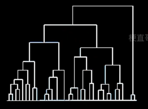
2.2、层次聚类
按照层次把数据划分到不同层的簇,形成树状结构,可以揭示数据间的分层结构
在树形结构上不同层次划分可以得到不同粒度的聚类
过程分为自底向上的聚合聚类和自顶向下的分裂聚类
自底向上的聚合聚类
将每个样本看做一个簇,初始状态下簇的数目 = 样本的数目
簇间距离最小的相似簇合并
下图纵轴不是合并的次序,而是合并的距离
簇间距离(簇间相似度)的度量
第一种 即使已经离得很近,可能也老死不能合并。
第二种 可能出现 链条式 的效果。
第三种 相对合适。

自顶向下的分裂聚类
所有样本看成一个簇
逐渐分裂成更小的簇
目前大多数聚类算法使用的都是自底向上的聚合聚类方法
3、聚类算法代码实现
import numpy as np
import matplotlib.pyplot as plt
from sklearn.datasets import make_blobs
X, y = make_blobs(n_samples=250, centers=5, n_features=2, random_state=0)
plt.scatter(X[:,0], X[:,1], c=y)
plt.show()
plt.scatter(X[:,0], X[:,1])
plt.show()
KMeans 聚类法
from sklearn.cluster import KMeans
kmeans = KMeans(n_clusters=5, random_state=0).fit(X)
此处设定簇的个数为5
kmeans.labels_注意,聚类不是分类,0-4只是相当于五个小组,治愈每个组是什么类型并不知道。
array([4, 4, 0, 1, 2, 0, 1, 0, 3, 2, 4, 0, 3, 2, 1, 2, 2, 4, 2, 0, 0, 0,
       4, 1, 1, 1, 0, 3, 4, 1, 0, 0, 2, 3, 4, 2, 2, 4, 2, 2, 4, 3, 1, 0,
       0, 3, 3, 2, 0, 1, 0, 1, 1, 1, 3, 2, 3, 4, 0, 0, 0, 3, 2, 3, 3, 0,
       4, 3, 4, 0, 0, 2, 4, 2, 1, 0, 2, 1, 1, 4, 1, 4, 0, 3, 2, 0, 3, 4,
       2, 3, 0, 3, 1, 0, 4, 1, 3, 2, 0, 2, 4, 3, 2, 0, 3, 3, 0, 4, 3, 0,
       0, 3, 3, 1, 3, 1, 0, 2, 3, 4, 4, 0, 2, 4, 3, 3, 4, 2, 2, 3, 4, 4,
       0, 2, 2, 4, 0, 1, 3, 3, 2, 0, 2, 1, 2, 3, 2, 0, 4, 0, 1, 0, 4, 3,
       1, 3, 3, 1, 3, 2, 2, 1, 1, 0, 1, 4, 0, 1, 2, 3, 3, 4, 2, 2, 0, 4,
       4, 1, 4, 2, 1, 3, 1, 1, 0, 4, 3, 1, 2, 1, 1, 2, 3, 4, 4, 2, 1, 2,
       1, 3, 4, 2, 1, 1, 1, 4, 3, 2, 0, 4, 3, 3, 2, 0, 3, 4, 4, 0, 3, 4,
       3, 2, 0, 1, 3, 3, 0, 0, 2, 2, 0, 2, 2, 1, 0, 1, 1, 4, 4, 1, 2, 1,
       4, 1, 4, 3, 4, 3, 1, 1], dtype=int32)
plt.scatter(X[:,0], X[:,1], c=kmeans.labels_)<matplotlib.collections.PathCollection at 0x7f3285fb57c0>

center = kmeans.cluster_centers_
center
array([[ 0.93226669, 4.273606 ],
[ 9.27996402, -2.3764533 ],
[ 2.05849588, 0.9767519 ],
[-1.39550161, 7.57857088],
[-1.85199006, 2.98013351]])
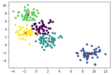
plt.scatter(X[:,0], X[:,1], c=kmeans.labels_)
center = kmeans.cluster_centers_
plt.scatter(center[:,0],center[:,1], marker='x', c = 'red')
plt.show()
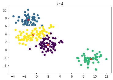
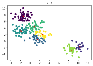
for n_clusters in [2, 3, 4, 5, 6, 7]:
    clusterer = KMeans(n_clusters=n_clusters, random_state=0).fit(X)
    z = clusterer.labels_
    center = clusterer.cluster_centers_
    plt.scatter(X[:,0], X[:,1], c=z)
    plt.scatter(center[:,0], center[:,1],marker = 'x', c='red')
    plt.title("k: {0}".format(n_clusters))
    plt.show()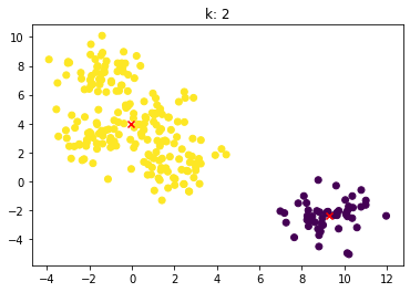


层次聚类法 没有聚类中心
from sklearn.cluster import AgglomerativeClustering
agg = AgglomerativeClustering(linkage='ward', n_clusters=5).fit(X)
plt.scatter(X[:,0], X[:,1], c=agg.labels_)
plt.show()
当我们对簇的个数没有预期时,不要一个一个试,可以传入距离的阈值。
agg = AgglomerativeClustering(distance_threshold=10, n_clusters=None).fit(X)
plt.scatter(X[:,0], X[:,1], c=agg.labels_)
plt.show()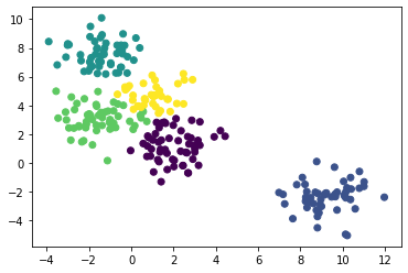
from scipy.cluster.hierarchy import linkage, dendrogram
def show_dendrogram(model):
    counts = np.zeros(model.children_.shape[0])
    n_samples = len(model.labels_)
    for i, merge in enumerate(model.children_):
        current_count = 0
        for child_idx in merge:
            if child_idx < n_samples:
                current_count += 1  # leaf node
            else:
                current_count += counts[child_idx - n_samples]
        counts[i] = current_count

    linkage_matrix = np.column_stack(
        [model.children_, model.distances_, counts]
    ).astype(float)
    dendrogram(linkage_matrix)
show_dendrogram(agg)
import time
import warnings

from sklearn import cluster, datasets
from sklearn.preprocessing import StandardScaler
from itertools import cycle, islice
n_samples = 1500
noisy_circles = datasets.make_circles(n_samples=n_samples, factor=0.5, noise=0.05)
noisy_moons = datasets.make_moons(n_samples=n_samples, noise=0.05)
blobs = datasets.make_blobs(n_samples=n_samples, random_state=8)
no_structure = np.random.rand(n_samples, 2), None

# Anisotropicly distributed data
random_state = 170
X, y = datasets.make_blobs(n_samples=n_samples, random_state=random_state)
transformation = [[0.6, -0.6], [-0.4, 0.8]]
X_aniso = np.dot(X, transformation)
aniso = (X_aniso, y)

# blobs with varied variances
varied = datasets.make_blobs(
    n_samples=n_samples, cluster_std=[1.0, 2.5, 0.5], random_state=random_state
)

# Set up cluster parameters
plt.figure(figsize=(9 * 1.3 + 2, 14.5))
plt.subplots_adjust(
    left=0.02, right=0.98, bottom=0.001, top=0.96, wspace=0.05, hspace=0.01
)

plot_num = 1

default_base = {"n_neighbors": 10, "n_clusters": 3}

datasets = [
    (noisy_circles, {"n_clusters": 2}),
    (noisy_moons, {"n_clusters": 2}),
    (varied, {"n_neighbors": 2}),
    (aniso, {"n_neighbors": 2}),
    (blobs, {}),
    (no_structure, {}),
]

for i_dataset, (dataset, algo_params) in enumerate(datasets):
    # update parameters with dataset-specific values
    params = default_base.copy()
    params.update(algo_params)

    X, y = dataset

    # normalize dataset for easier parameter selection
    X = StandardScaler().fit_transform(X)

    # ============
    # Create cluster objects
    # ============
    ward = cluster.AgglomerativeClustering(
        n_clusters=params["n_clusters"], linkage="ward"
    )
    complete = cluster.AgglomerativeClustering(
        n_clusters=params["n_clusters"], linkage="complete"
    )
    average = cluster.AgglomerativeClustering(
        n_clusters=params["n_clusters"], linkage="average"
    )
    single = cluster.AgglomerativeClustering(
        n_clusters=params["n_clusters"], linkage="single"
    )

    clustering_algorithms = (
        ("Single Linkage", single),
        ("Average Linkage", average),
        ("Complete Linkage", complete),
        ("Ward Linkage", ward),
    )

    for name, algorithm in clustering_algorithms:
        t0 = time.time()

        # catch warnings related to kneighbors_graph
        with warnings.catch_warnings():
            warnings.filterwarnings(
                "ignore",
                message="the number of connected components of the "
                + "connectivity matrix is [0-9]{1,2}"
                + " > 1. Completing it to avoid stopping the tree early.",
                category=UserWarning,
            )
            algorithm.fit(X)

        t1 = time.time()
        if hasattr(algorithm, "labels_"):
            y_pred = algorithm.labels_.astype(int)
        else:
            y_pred = algorithm.predict(X)

        plt.subplot(len(datasets), len(clustering_algorithms), plot_num)
        if i_dataset == 0:
            plt.title(name, size=18)

        colors = np.array(
            list(
                islice(
                    cycle(
                        [
                            "#377eb8",
                            "#ff7f00",
                            "#4daf4a",
                            "#f781bf",
                            "#a65628",
                            "#984ea3",
                            "#999999",
                            "#e41a1c",
                            "#dede00",
                        ]
                    ),
                    int(max(y_pred) + 1),
                )
            )
        )
        plt.scatter(X[:, 0], X[:, 1], s=10, color=colors[y_pred])

        plt.xlim(-2.5, 2.5)
        plt.ylim(-2.5, 2.5)
        plt.xticks(())
        plt.yticks(())
        plt.text(
            0.99,
            0.01,
            ("%.2fs" % (t1 - t0)).lstrip("0"),
            transform=plt.gca().transAxes,
            size=15,
            horizontalalignment="right",
        )
        plot_num += 1

plt.show()
4、聚类评估代码实现
聚类效果评估方法
已知标签评价
调整兰德指数Adjusted Rand lndex
调整互信息分Adjusted mutual info score
基于预测簇向量与真实簇向量的互信息分数
V-Measure
同质性和完整性的调和平均值
————取值在-1到1,越接近1越好
未知标签评价
轮廓系数
通过计算样本与所在簇中其他样本的相似度
CHI (Calinski-Harabaz lndex/Variance Ratio Criterion)
群间离散度和群内离散度的比例
代码实现
import numpy as np
import matplotlib.pyplot as plt
from sklearn.datasets import make_blobs
X, y = make_blobs(n_samples=250, n_features=2, centers=5, random_state=0)from sklearn.cluster import KMeans
kmeans = KMeans(n_clusters=5, random_state=0).fit(X)
z = kmeans.labels_center = kmeans.cluster_centers_
plt.scatter(X[:,0], X[:,1], c=z)
plt.scatter(center[:,0], center[:,1], marker = 'x', c='red')
plt.show()
已知标签
from sklearn.metrics import adjusted_rand_score
adjusted_rand_score(y,z)
0.8676297613641788
from sklearn.metrics import adjusted_mutual_info_score
adjusted_mutual_info_score(y,z)
0.8579576361507845
from sklearn.metrics import v_measure_score
v_measure_score(y,z)
0.8608558483955058
ari_curve = []
ami_curve = []
vm_curve = []
clus = [2, 3, 4, 5, 6, 7]
for n_clusters in clus:
    clusterer = KMeans(n_clusters=n_clusters, random_state=0).fit(X)
    z = clusterer.labels_
    ari_curve.append(adjusted_rand_score(y,z))
    ami_curve.append(adjusted_mutual_info_score(y,z))
    vm_curve.append(v_measure_score(y,z))

plt.plot(clus, ari_curve, label='ari')
plt.plot(clus, ami_curve, label='ami')
plt.plot(clus, vm_curve, label='vm')
plt.legend()
plt.show()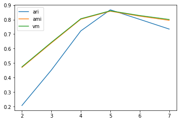
未知标签
from sklearn.metrics import silhouette_score
kmeans = KMeans(n_clusters=5, random_state=0).fit(X)
cluster_labels = kmeans.labels_
si = silhouette_score(X, cluster_labels)
si
0.5526930597314647
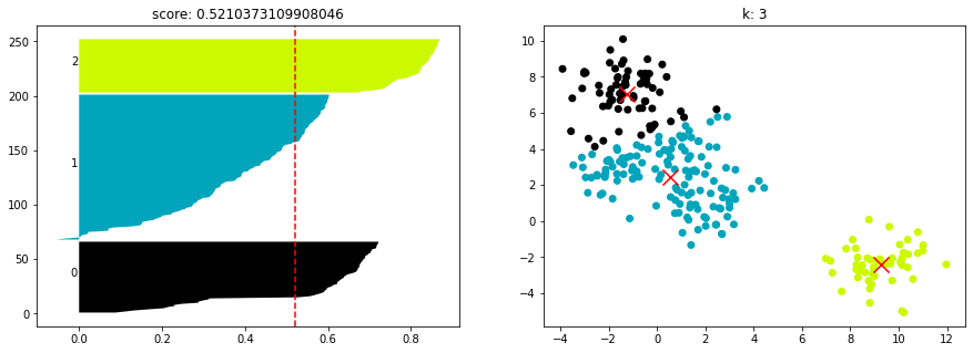
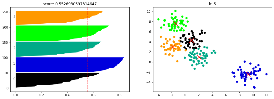
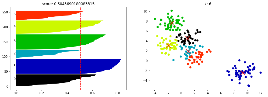
from sklearn.metrics import silhouette_samples
import matplotlib.cm as cm

def show_silhouette_plot(model, X):
    for n_clusters in [2, 3, 4, 5, 6, 7]:
        fig, (pic1, pic2) = plt.subplots(1, 2)
        fig.set_size_inches(15, 5)
        model.n_clusters = n_clusters
        clusterer = model.fit(X)
        cluster_labels = clusterer.labels_
        centers = clusterer.cluster_centers_
        silhouette_avg = silhouette_score(X, cluster_labels)
        sample_silhouette_values = silhouette_samples(X, cluster_labels)

        y_lower = 1
        for i in range(n_clusters):
            ith_cluster_silhouette_values = sample_silhouette_values[cluster_labels == i]
            ith_cluster_silhouette_values.sort()
            size_cluster_i = ith_cluster_silhouette_values.shape[0]
            y_upper = y_lower + size_cluster_i
            color = cm.nipy_spectral(float(i) / n_clusters)
            pic1.fill_betweenx(np.arange(y_lower, y_upper), ith_cluster_silhouette_values, facecolor = color)
            pic1.text(-0.02, y_lower + 0.5 * size_cluster_i, str(i))
            y_lower = y_upper + 1

        pic1.axvline(x = silhouette_avg, color = 'red', linestyle = "--")
        pic1.set_title("score: {0}".format(silhouette_avg))

        colors = cm.nipy_spectral(cluster_labels.astype(float) / n_clusters)
        pic2.scatter(X[:,0], X[:,1], marker = 'o', c = colors)
        pic2.scatter(centers[:, 0], centers[:, 1], marker = 'x', c = 'red', alpha = 1, s = 200)
        pic2.set_title("k: {0}".format(n_clusters))
show_silhouette_plot(kmeans, X)


from sklearn.metrics import calinski_harabasz_score
calinski_harabasz_score(X, y)
850.6346471314978
chi_curve = []

clus = [2, 3, 4, 5, 6, 7]
for n_clusters in clus:
    clusterer = KMeans(n_clusters=n_clusters, random_state=0).fit(X)
    z = clusterer.labels_
    chi_curve.append(calinski_harabasz_score(X,z))

plt.plot(clus, chi_curve, label='chi')
plt.legend()
plt.show()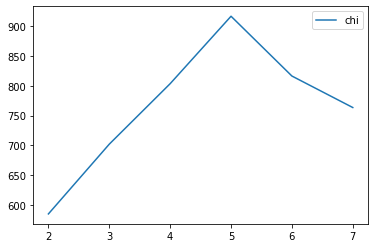
5、优缺点和适用条件
K--means聚类优缺点
优点
算法简单,收敛速度快
簇间区别大时效果好
对大数据集,算法可伸缩性强(可伸缩性:但数据从几百上升到几百万时,聚类结果的准确度/一致性 特别好)
缺点
簇数k难以估计
对初始聚类中心敏感
容易陷入局部最优
簇不规则时,容易对大簇分割(当采用误差平方和的准则作为聚类准则函数,如果各类的大小或形状差距很大时,有可能出现将大类分割的现象)
‘
’K--means聚类适用条件
簇是密集的、球状或团状
簇与簇间区别明显
簇本身数据比较均匀
适用大数据集
凸性簇
分层聚类优缺点
优点
距离相似度容易定义限制少
无需指定簇数
可以发现簇的层次关系
缺点
由于要计算邻近度矩阵,对时间和空间需求大
困难在于合并或分裂点的选择
可拓展性差
分层聚类适用条件
适合于小型数据集的聚类
可以在不同粒度水平上对数据进行探测,发现簇间层次关系
参考
Machine-Learning: 《机器学习必修课:经典算法与Python实战》配套代码 - Gitee.com