注意力机制
在整个注意力过程中,模型会学习了三个权重:查询、键和值。查询、键和值的思想来源于信息检索系统。所以我们先理解数据库查询的思想。
假设有一个数据库,里面有所有一些作家和他们的书籍信息。现在我想读一些Rabindranath写的书:
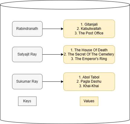
在数据库中,作者名字类似于键,图书类似于值。查询的关键词Rabindranath是这个问题的键。所以需要计算查询和数据库的键(数据库中的所有作者)之间的相似度,然后返回最相似作者的值(书籍)。
同样,注意力有三个矩阵,分别是查询矩阵(Q)、键矩阵(K)和值矩阵(V)。它们中的每一个都具有与输入嵌入相同的维数。模型在训练中学习这些度量的值。
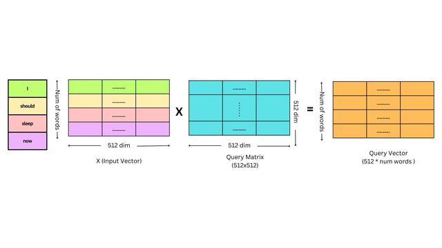
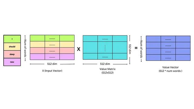
我们可以假设我们从每个单词中创建一个向量,这样我们就可以处理信息。对于每个单词,生成一个512维的向量。所有3个矩阵都是512x512(因为单词嵌入的维度是512)。对于每个标记嵌入,我们将其与所有三个矩阵(Q, K, V)相乘,每个标记将有3个长度为512的中间向量。
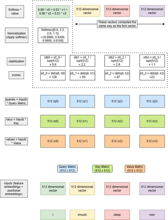
接下来计算分数,它是查询和键向量之间的点积。分数决定了当我们在某个位置编码单词时,对输入句子的其他部分的关注程度。
然后将点积除以关键向量维数的平方根。这种缩放是为了防止点积变得太大或太小(取决于正值或负值),因为这可能导致训练期间的数值不稳定。选择比例因子是为了确保点积的方差近似等于1。
然后通过softmax操作传递结果。这将分数标准化:它们都是正的,并且加起来等于1。softmax输出决定了我们应该从不同的单词中获取多少信息或特征(值),也就是在计算权重。
这里需要注意的一点是,为什么需要其他单词的信息/特征?因为我们的语言是有上下文含义的,一个相同的单词出现在不同的语境,含义也不一样。
最后一步就是计算softmax与这些值的乘积,并将它们相加。
可视化图解
上面逻辑都是文字内容,看起来有一些枯燥,下面我们可视化它的矢量化实现。这样可以更加深入的理解。
查询键和矩阵的计算方法如下
同样的方法可以计算键向量和值向量。

最后计算得分和注意力输出。

简单代码实现
import torch
import torch.nn as nn
from typing import List
def get_input_embeddings(words: List[str], embeddings_dim: int):
# we are creating random vector of embeddings_dim size for each words
# normally we train a tokenizer to get the embeddings.
# check the blog on tokenizer to learn about this part
embeddings = [torch.randn(embeddings_dim) for word in words]
return embeddings
text = "I should sleep now"
words = text.split(" ")
len(words) # 4
embeddings_dim = 512 # 512 dim because the original paper uses it. we can use other dim also
embeddings = get_input_embeddings(words, embeddings_dim=embeddings_dim)
embeddings[0].shape # torch.Size([512])
# initialize the query, key and value metrices
query_matrix = nn.Linear(embeddings_dim, embeddings_dim)
key_matrix = nn.Linear(embeddings_dim, embeddings_dim)
value_matrix = nn.Linear(embeddings_dim, embeddings_dim)
query_matrix.weight.shape, key_matrix.weight.shape, value_matrix.weight.shape # torch.Size([512, 512]), torch.Size([512, 512]), torch.Size([512, 512])
# query, key and value vectors computation for each words embeddings
query_vectors = torch.stack([query_matrix(embedding) for embedding in embeddings])
key_vectors = torch.stack([key_matrix(embedding) for embedding in embeddings])
value_vectors = torch.stack([value_matrix(embedding) for embedding in embeddings])
query_vectors.shape, key_vectors.shape, value_vectors.shape # torch.Size([4, 512]), torch.Size([4, 512]), torch.Size([4, 512])
# compute the score
scores = torch.matmul(query_vectors, key_vectors.transpose(-2, -1)) / torch.sqrt(torch.tensor(embeddings_dim, dtype=torch.float32))
scores.shape # torch.Size([4, 4])
# compute the attention weights for each of the words with the other words
softmax = nn.Softmax(dim=-1)
attention_weights = softmax(scores)
attention_weights.shape # torch.Size([4, 4])
# attention output
output = torch.matmul(attention_weights, value_vectors)
output.shape # torch.Size([4, 512])
以上代码只是为了展示注意力机制的实现,并未优化。
多头注意力
上面提到的注意力是单头注意力,在原论文中有8个头。对于多头和单多头注意力计算相同,只是查询(q0-q3),键(k0-k3),值(v0-v3)中间向量会有一些区别。
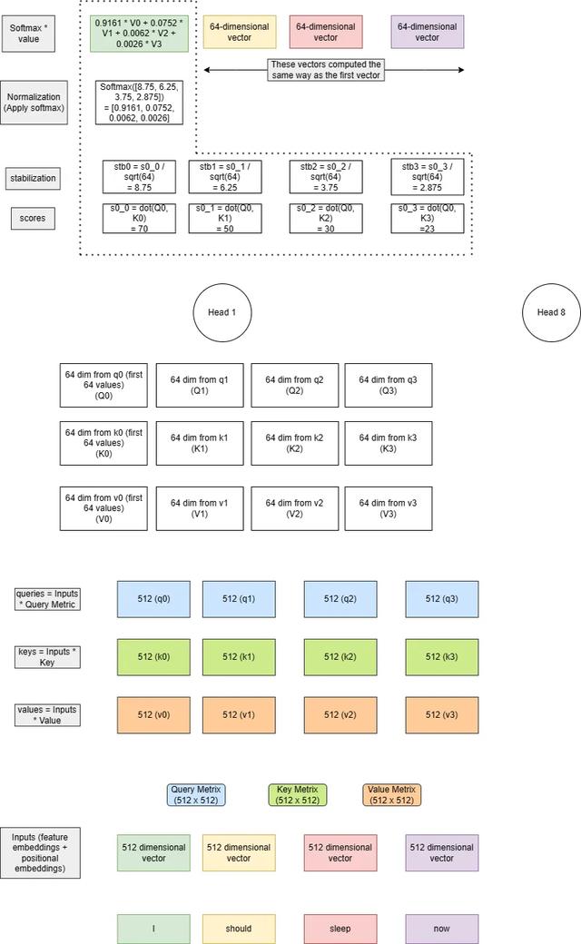
之后将查询向量分成相等的部分(有多少头就分成多少)。在上图中有8个头,查询,键和值向量的维度为512。所以就变为了8个64维的向量。
把前64个向量放到第一个头,第二组向量放到第二个头,以此类推。在上面的图片中,我只展示了第一个头的计算。
这里需要注意的是:不同的框架有不同的实现方法,pytorch官方的实现是上面这种,但是tf和一些第三方的代码中是将每个头分开计算了,比如8个头会使用8个linear(tf的dense)而不是一个大linear再拆解。还记得Pytorch的transformer里面要求emb_dim能被num_heads整除吗,就是因为这个
使用哪种方式都可以,因为最终的结果都类似影响不大。
当我们在一个head中有了小查询、键和值(64 dim的)之后,计算剩下的逻辑与单个head注意相同。最后得到的64维的向量来自每个头。
我们将每个头的64个输出组合起来,得到最后的512个dim输出向量。
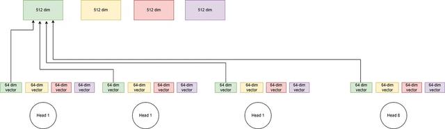
多头注意力可以表示数据中的复杂关系。每个头都能学习不同的模式。多个头还提供了同时处理输入表示的不同子空间(本例:64个向量表示512个原始向量)的能力。
多头注意代码实现
num_heads = 8
# batch dim is 1 since we are processing one text.
batch_size = 1
text = "I should sleep now"
words = text.split(" ")
len(words) # 4
embeddings_dim = 512
embeddings = get_input_embeddings(words, embeddings_dim=embeddings_dim)
embeddings[0].shape # torch.Size([512])
# initialize the query, key and value metrices
query_matrix = nn.Linear(embeddings_dim, embeddings_dim)
key_matrix = nn.Linear(embeddings_dim, embeddings_dim)
value_matrix = nn.Linear(embeddings_dim, embeddings_dim)
query_matrix.weight.shape, key_matrix.weight.shape, value_matrix.weight.shape # torch.Size([512, 512]), torch.Size([512, 512]), torch.Size([512, 512])
# query, key and value vectors computation for each words embeddings
query_vectors = torch.stack([query_matrix(embedding) for embedding in embeddings])
key_vectors = torch.stack([key_matrix(embedding) for embedding in embeddings])
value_vectors = torch.stack([value_matrix(embedding) for embedding in embeddings])
query_vectors.shape, key_vectors.shape, value_vectors.shape # torch.Size([4, 512]), torch.Size([4, 512]), torch.Size([4, 512])
# (batch_size, num_heads, seq_len, embeddings_dim)
query_vectors_view = query_vectors.view(batch_size, -1, num_heads, embeddings_dim//num_heads).transpose(1, 2)
key_vectors_view = key_vectors.view(batch_size, -1, num_heads, embeddings_dim//num_heads).transpose(1, 2)
value_vectors_view = value_vectors.view(batch_size, -1, num_heads, embeddings_dim//num_heads).transpose(1, 2)
query_vectors_view.shape, key_vectors_view.shape, value_vectors_view.shape
# torch.Size([1, 8, 4, 64]),
# torch.Size([1, 8, 4, 64]),
# torch.Size([1, 8, 4, 64])
# We are splitting the each vectors into 8 heads.
# Assuming we have one text (batch size of 1), So we split
# the embedding vectors also into 8 parts. Each head will
# take these parts. If we do this one head at a time.
head1_query_vector = query_vectors_view[0, 0, ...]
head1_key_vector = key_vectors_view[0, 0, ...]
head1_value_vector = value_vectors_view[0, 0, ...]
head1_query_vector.shape, head1_key_vector.shape, head1_value_vector.shape
# The above vectors are of same size as before only the feature dim is changed from 512 to 64
# compute the score
scores_head1 = torch.matmul(head1_query_vector, head1_key_vector.permute(1, 0)) / torch.sqrt(torch.tensor(embeddings_dim//num_heads, dtype=torch.float32))
scores_head1.shape # torch.Size([4, 4])
# compute the attention weights for each of the words with the other words
softmax = nn.Softmax(dim=-1)
attention_weights_head1 = softmax(scores_head1)
attention_weights_head1.shape # torch.Size([4, 4])
output_head1 = torch.matmul(attention_weights_head1, head1_value_vector)
output_head1.shape # torch.Size([4, 512])
# we can compute the output for all the heads
outputs = []
for head_idx in range(num_heads):
head_idx_query_vector = query_vectors_view[0, head_idx, ...]
head_idx_key_vector = key_vectors_view[0, head_idx, ...]
head_idx_value_vector = value_vectors_view[0, head_idx, ...]
scores_head_idx = torch.matmul(head_idx_query_vector, head_idx_key_vector.permute(1, 0)) / torch.sqrt(torch.tensor(embeddings_dim//num_heads, dtype=torch.float32))
softmax = nn.Softmax(dim=-1)
attention_weights_idx = softmax(scores_head_idx)
output = torch.matmul(attention_weights_idx, head_idx_value_vector)
outputs.append(output)
[out.shape for out in outputs]
# [torch.Size([4, 64]),
# torch.Size([4, 64]),
# torch.Size([4, 64]),
# torch.Size([4, 64]),
# torch.Size([4, 64]),
# torch.Size([4, 64]),
# torch.Size([4, 64]),
# torch.Size([4, 64])]
# stack the result from each heads for the corresponding words
word0_outputs = torch.cat([out[0] for out in outputs])
word0_outputs.shape
# lets do it for all the words
attn_outputs = []
for i in range(len(words)):
attn_output = torch.cat([out[i] for out in outputs])
attn_outputs.append(attn_output)
[attn_output.shape for attn_output in attn_outputs] # [torch.Size([512]), torch.Size([512]), torch.Size([512]), torch.Size([512])]
# Now lets do it in vectorize way.
# We can not permute the last two dimension of the key vector.
key_vectors_view.permute(0, 1, 3, 2).shape # torch.Size([1, 8, 64, 4])
# Transpose the key vector on the last dim
score = torch.matmul(query_vectors_view, key_vectors_view.permute(0, 1, 3, 2)) # Q*k
score = torch.softmax(score, dim=-1)
# reshape the results
attention_results = torch.matmul(score, value_vectors_view)
attention_results.shape # [1, 8, 4, 64]
# merge the results
attention_results = attention_results.permute(0, 2, 1, 3).contiguous().view(batch_size, -1, embeddings_dim)
attention_results.shape # torch.Size([1, 4, 512])
总结
注意力机制(attention mechanism)是Transformer模型中的重要组成部分。Transformer是一种基于自注意力机制(self-attention)的神经网络模型,广泛应用于自然语言处理任务,如机器翻译、文本生成和语言模型等。本文介绍的自注意力机制是Transformer模型的基础,在此基础之上衍生发展出了各种不同的更加高效的注意力机制,所以深入了解自注意力机制,将能够更好地理解Transformer模型的设计原理和工作机制,以及如何在具体的各种任务中应用和调整模型。这将有助于你更有效地使用Transformer模型并进行相关研究和开发。
原文出处,入侵吾删