TensorFlow中5个不同的层次结构：即硬件层，内核层，低阶API，中阶API，高阶API。本文以线性回归和DNN二分类模型为例，直观对比展示在不同层级实现模型的特点。

Tensorflow的层次结构

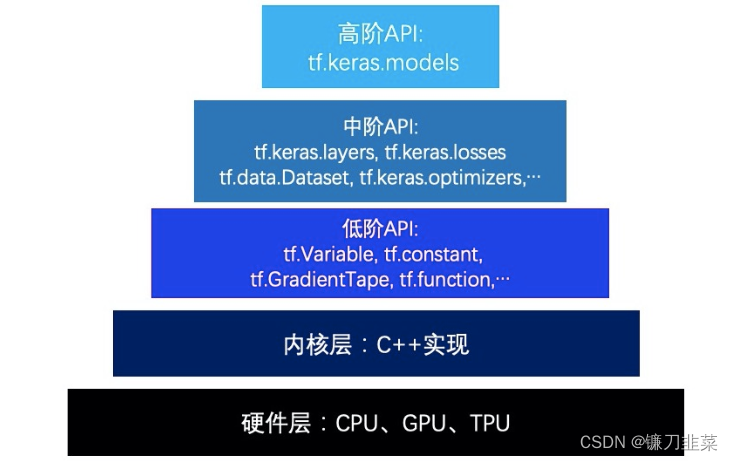
TensorFlow的层次结构从低到高可以分成如下五层：

• 最底层为硬件层，TensorFlow支持CPU、GPU或TPU加入计算资源池。
• 第二层为C++实现的内核，kernel可以跨平台分布运行。
• 第三层为Python实现的操作符，提供了封装C++内核的低级API指令，主要包括各种张量操作算子、计算图、自动微分。如tf.Variable,tf.constant,tf.function,tf.GradientTape,tf.nn.softmax… 如果把模型比作一个房子，那么第三层API就是模型之砖。
• 第四层为Python实现的模型组件，对低级API进行了函数封装，主要包括各种模型层，损失函数，优化器，数据管道，特征列等等。如tf.keras.layers,tf.keras.losses,tf.keras.metrics,tf.keras.optimizers,tf.data.DataSet,tf.feature_column…如果把模型比作一个房子，那么第四层API就是模型之墙。
• 第五层为Python实现的模型成品，一般为按照OOP方式封装的高级API，主要为tf.keras.models提供的模型的类接口。如果把模型比作一个房子，那么第五层API就是模型本身，即模型之屋。

Tensorflow的低阶API示例

低阶API主要包括张量操作，计算图和自动微分。

import tensorflow as tf


#打印时间分割线
@tf.function
def printbar():
    today_ts = tf.timestamp() % (24 * 60 * 60)

    hour = tf.cast(today_ts // 3600 + 8, tf.int32) % tf.constant(24)
    minite = tf.cast((today_ts % 3600) // 60, tf.int32)
    second = tf.cast(tf.floor(today_ts % 60), tf.int32)

    def timeformat(m):
        if tf.strings.length(tf.strings.format("{}", m)) == 1:
            return (tf.strings.format("0{}", m))
        else:
            return (tf.strings.format("{}", m))

    timestring = tf.strings.join([timeformat(hour), timeformat(minite), timeformat(second)], separator=":")
    tf.print("==========" * 8 + timestring)

下面使用TensorFlow的低阶API实现线性回归模型和DNN二分类模型：

线性回归模型

准备数据

import numpy as np
import pandas as pd
from matplotlib import pyplot as plt
import tensorflow as tf

# 样本数量
n = 400
# 生成测试用数据集
X= tf.random.uniform([n,2], minval=-10, maxval=10)
w0 = tf.constant([[2.0], [-3.0]])
b0 = tf.constant([[3.0]])

# @表示矩阵惩罚，并增加正态扰动
Y = X@w0+b0+tf.random.normal([n,1],mean=0.0, stddev=2.0)

数据可视化：

%matplotlib inline
%config InlineBackend.figure_format = 'svg'
# 数据可视化
plt.figure(figsize=(12, 5))
ax1 = plt.subplot(121)
ax1.scatter(X[:,0], Y[:,0], c='b')
plt.xlabel('x1')
plt.ylabel('y', rotation = 0)

ax2 = plt.subplot(122)
ax2.scatter(X[:,1],Y[:,0],c='g')
plt.xlabel('x2')
plt.ylabel('y', rotation=0)
plt.show()

构建数据管道迭代器：

def data_iter(features, labels, batch_size=8):
    num_examples = len(features)
    indices = list(range(num_examples))
    np.random.shuffle(indices) # 样本的读取顺序是随机的
    for i in range(0, num_examples, batch_size):
        indexs = indices[i: min(i + batch_size, num_examples)]
        yield tf.gather(features,indexs), tf.gather(labels, indexs)

# 测试数据管道效果
batch_size = 8
(features, labels) = next(data_iter(X, Y, batch_size))
print(features)
print(labels)

数据管道效果：

tf.Tensor(
[[-5.076039   -0.9657364 ]
 [-6.358912   -3.6004496 ]
 [-7.056513   -3.9889216 ]
 [ 2.3329067  -2.8891182 ]
 [-5.9270716  -8.905029  ]
 [-0.16547203 -3.6211562 ]
 [ 6.9834538  -1.579752  ]
 [-5.3834534   2.5390549 ]], shape=(8, 2), dtype=float32)
tf.Tensor(
[[ -1.4625118]
 [  1.6316607]
 [  2.0894573]
 [ 12.264805 ]
 [ 16.555326 ]
 [ 10.086447 ]
 [ 21.4322   ]
 [-14.078172 ]], shape=(8, 1), dtype=float32)

定义模型

w = tf.Variable(tf.random.normal(w0.shape))
b = tf.Variable(tf.zeros_like(b0, dtype=tf.float32))


# 定义模型
class LinearRegression:
    # 正向传播
    def __call__(self, x):
        return x @ w + b

    # 损失函数
    def loss_func(self, y_true, y_pred):
        return tf.reduce_mean((y_true - y_pred) ** 2 / 2)


model = LinearRegression()

训练模型

1. 使用动态图调试

# 使用动态图调试
def train_step(model, features, labels):
    with tf.GradientTape() as tape:
        predictions = model(features)
        loss = model.loss_func(labels, predictions)
    # 反向传播求梯度
    dloss_dw, dloss_db = tape.gradient(loss, [w, b])
    # 梯度下降法更新参数
    w.assign(w - 0.001*dloss_dw)
    b.assign(b - 0.001*dloss_db)
    return loss

测试train_step效果：

batch_size = 10
(features, labels) = next(data_iter(X, Y, batch_size))
train_step(model, features, labels)
'''
<tf.Tensor: shape=(), dtype=float32, numpy=277.26096>
'''

定义模型训练函数：

def train_model(model, epochs):
    for epoch in tf.range(1, epochs+1):
        for features, labels in data_iter(X, Y, 10):
            loss = train_step(model, features, labels)

        if epoch%50==0:
            tf.print('=========='*8)
            tf.print('epoch =',epoch, "loss = ",loss)
            tf.print('w = ',w)
            tf.print('b = ',b)

train_model(model, epochs=200)

训练过程：

================================================================================
epoch = 50 loss =  0.846690834
w =  [[1.99412823]
 [-2.99952745]]
b =  [[3.04354715]]
================================================================================
epoch = 100 loss =  1.1837182
w =  [[1.99304128]
 [-2.99331546]]
b =  [[3.04392529]]
================================================================================
epoch = 150 loss =  1.58060181
w =  [[1.99656463]
 [-2.98927522]]
b =  [[3.04404855]]
================================================================================
epoch = 200 loss =  2.5443294
w =  [[2.00231266]
 [-2.97837281]]
b =  [[3.04363918]]

2. 使用autograph机制转换成静态图加速

@tf.function
def train_step(model, features, labels):
    with tf.GradientTape() as tape:
        predictions = model(features)
        loss = model.loss_func(labels, predictions)
    # 反向传播求梯度
    dloss_dw, dloss_db = tape.gradient(loss, [w, b])
    # 梯度下降法更新参数
    w.assign(w - 0.001 * dloss_dw)
    b.assign(b - 0.001 * dloss_db)

    return loss


def train_model(model, epochs):
    for epoch in tf.range(1, epochs + 1):
        for features, labels in data_iter(X, Y, 10):
            loss = train_step(model, features, labels)
        if epoch % 50 == 0:
            tf.print('=========='*8)
            tf.print("epoch =", epoch, "loss = ", loss)
            tf.print("w =", w)
            tf.print("b =", b)


train_model(model, epochs=200)

训练过程：

================================================================================
epoch = 50 loss =  1.16669047
w = [[1.99806643]
 [-2.99671936]]
b = [[3.04368925]]
================================================================================
epoch = 100 loss =  1.40429044
w = [[2.00206447]
 [-2.98451281]]
b = [[3.04383779]]
================================================================================
epoch = 150 loss =  1.7426182
w = [[1.98978758]
 [-2.99107504]]
b = [[3.04403]]
================================================================================
epoch = 200 loss =  2.16272426
w = [[1.99508071]
 [-2.98746681]]
b = [[3.04382515]]

结果可视化：

%matplotlib inline
%config InlineBackend.figure_format = 'svg'

plt.figure(figsize=(12, 5))
ax1 = plt.subplot(121)
ax1.scatter(X[:, 0], Y[:, 0], c="b", label="samples")
ax1.plot(X[:, 0], w[0] * X[:, 0] + b[0], "-r", linewidth=5.0, label="model")
ax1.legend()
plt.xlabel("x1")
plt.ylabel("y", rotation=0)

ax2 = plt.subplot(122)
ax2.scatter(X[:, 1], Y[:, 0], c="g", label="samples")
ax2.plot(X[:, 1], w[1] * X[:, 1] + b[0], "-r", linewidth=5.0, label="model")
ax2.legend()
plt.xlabel("x2")
plt.ylabel("y", rotation=0)

plt.show()

DNN二分类模型

准备数据

import pandas as pd
import numpy as np
import matplotlib.pyplot as plt
import tensorflow as tf

配置notebook的cell：

%matplotlib inline
%config InlineBackend.figure_format = 'svg'

生成正负样本：

# 正负样本数量
n_positive, n_negative = 2000, 2000

# 生成正样本，小圆环分布
r_p = 5.0 + tf.random.truncated_normal([n_positive,1], 0.0, 1.0)
theta_p = tf.random.uniform([n_positive,1], 0.0, 2*np.pi)
Xp = tf.concat([r_p*tf.cos(theta_p), r_p*tf.sin(theta_p)], axis=1)
Yp = tf.ones_like(r_p)

# 生成负样本， 大圆环分布
r_n = 8.0 + tf.random.truncated_normal([n_negative, 1], 0.0, 1.0)
theta_n = tf.random.uniform([n_negative, 1], 0.0, 2*np.pi)
Xn = tf.concat([r_n*tf.cos(theta_n), r_n*tf.sin(theta_n)], axis=1)
Yn = tf.zeros_like(r_n)

# 汇总数据
X = tf.concat([Xp, Xn], axis=0)
Y = tf.concat([Yp, Yn], axis=0)

可视化数据：

# 可视化
plt.figure(figsize=(6,6))
plt.scatter(Xp[:,0].numpy(), Xp[:,1].numpy(), c='r')
plt.scatter(Xn[:,0].numpy(), Xn[:,1].numpy(), c='g')
plt.legend(['positive','negative'])

构建数据管道迭代器：

# 构建数据管道迭代器
def data_iter(features, labels, batch_size=8):
    num_examples = len(features)
    indices = list(range(num_examples))
    np.random.shuffle(indices)  #样本的读取顺序是随机的
    for i in range(0, num_examples, batch_size):
        indexs = indices[i: min(i + batch_size, num_examples)]
        yield tf.gather(features,indexs), tf.gather(labels,indexs)

# 测试数据管道效果
batch_size = 10
(features, labels) = next(data_iter(X, Y, batch_size))
print(features)
print(labels)

定义模型

这里利用tf.Module来组织模型变量:

class DNNModel(tf.Module):
    def __init__(self, name=None):
        super(DNNModel, self).__init__(name=name)
        self.w1 = tf.Variable(tf.random.truncated_normal([2, 4]), dtype=tf.float32)
        self.b1 = tf.Variable(tf.zeros([1, 4]), dtype=tf.float32)
        self.w2 = tf.Variable(tf.random.truncated_normal([4, 8]), dtype=tf.float32)
        self.b2 = tf.Variable(tf.zeros([1, 8]), dtype=tf.float32)
        self.w3 = tf.Variable(tf.random.truncated_normal([8, 1]), dtype=tf.float32)
        self.b3 = tf.Variable(tf.zeros([1, 1]), dtype=tf.float32)

    # 正向传播
    @tf.function(input_signature=[tf.TensorSpec(shape=[None, 2], dtype=tf.float32)])
    def __call__(self, x):
        x = tf.nn.relu(x @ self.w1 + self.b1)
        x = tf.nn.relu(x @ self.w2 + self.b2)
        y = tf.nn.sigmoid(x @ self.w3 + self.b3)
        return y

    # 损失函数（二元交叉熵）
    @tf.function(input_signature=[tf.TensorSpec(shape=[None, 1], dtype=tf.float32),
                                  tf.TensorSpec(shape=[None, 1], dtype=tf.float32)])
    def loss_func(self, y_true, y_pred):
        # 将预测值限制在1e-7以下， 1-1e-7以下，避免log(0)错误
        eps = 1e-7
        y_pred = tf.clip_by_value(y_pred, eps, 1.0 - eps)
        bce = -y_true * tf.math.log(y_pred) - (1 - y_true) * tf.math.log(1 - y_pred)
        return tf.reduce_mean(bce)

    # 评估指标（准确率）
    @tf.function(input_signature=[tf.TensorSpec(shape=[None, 1], dtype=tf.float32),
                                  tf.TensorSpec(shape=[None, 1], dtype=tf.float32)])
    def metric_func(self, y_true, y_pred):
        y_pred = tf.where(y_pred > 0.5, tf.ones_like(y_pred, dtype=tf.float32), tf.zeros_like(y_pred, dtype=tf.float32))
        acc = tf.reduce_mean(1 - tf.abs(y_true - y_pred))
        return acc


model = DNNModel()

测试模型结构：

batch_size = 10
(features, labels) = next(data_iter(X, Y, batch_size))

predictions = model(features)

loss = model.loss_func(labels, predictions)
metric = model.metric_func(labels, predictions)

tf.print("init loss:", loss)
tf.print("init metric", metric)
'''
init loss: 0.475380838
init metric 0.8
'''
print(len(model.trainable_variables)) # 6

训练模型

使用autograph机制转换成静态图加速：

@tf.function
def train_step(model, features, labels):
    # 正向传播，计算损失
    with tf.GradientTape() as tape:
        predictions = model(features)
        loss = model.loss_func(labels, predictions)
    # 反向传播，计算梯度
    grads = tape.gradient(loss, model.trainable_variables)
    # 执行梯度下降
    for p, dloss_dp in zip(model.trainable_variables, grads):
        p.assign(p - 0.001 * dloss_dp)

    # 计算评估指标
    metric = model.metric_func(labels, predictions)
    return loss, metric


def train_model(model, epochs):
    for epoch in tf.range(1, epochs + 1):
        for features, labels in data_iter(X, Y, 100):
            loss, metric = train_step(model, features, labels)
        if epoch % 100 == 0:
            print('======='*10)
            tf.print("epoch =", epoch, "loss = ", loss, "accuracy = ", metric)


train_model(model, epochs=600)

训练记录：

======================================================================
epoch = 100 loss =  0.544845939 accuracy =  0.79
======================================================================
epoch = 200 loss =  0.475 accuracy =  0.85
======================================================================
epoch = 300 loss =  0.391879201 accuracy =  0.88
======================================================================
epoch = 400 loss =  0.378405839 accuracy =  0.92
======================================================================
epoch = 500 loss =  0.289739966 accuracy =  0.98
======================================================================
epoch = 600 loss =  0.310408324 accuracy =  0.87

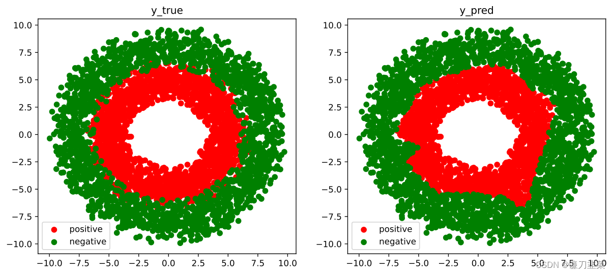
结果可视化：

fig, (ax1, ax2) = plt.subplots(nrows=1, ncols=2, figsize=(12, 5))
ax1.scatter(Xp[:, 0], Xp[:, 1], c="r")
ax1.scatter(Xn[:, 0], Xn[:, 1], c="g")
ax1.legend(["positive", "negative"]);
ax1.set_title("y_true");

Xp_pred = tf.boolean_mask(X, tf.squeeze(model(X) >= 0.5), axis=0)
Xn_pred = tf.boolean_mask(X, tf.squeeze(model(X) < 0.5), axis=0)

ax2.scatter(Xp_pred[:, 0], Xp_pred[:, 1], c="r")
ax2.scatter(Xn_pred[:, 0], Xn_pred[:, 1], c="g")
ax2.legend(["positive", "negative"]);
ax2.set_title("y_pred");

Tensorflow的中阶API示例

TensorFlow的中阶API主要包括各种模型层，损失函数，优化器，数据管道，特征列等。

线性回归模型

构建输入数据管道

ds = tf.data.Dataset.from_tensor_slices((X, Y)).shuffle(buffer_size=100).batch(10).prefetch(tf.data.experimental.AUTOTUNE)

定义模型

from tensorflow.keras import layers,losses,metrics,optimizers

model = layers.Dense(units=1)
model.build(input_shape=(2,)) # 用build方法创建variables
model.loss_func = losses.mean_squared_error
model.optimizer = optimizers.SGD(learning_rate=0.001)

训练模型：
使用autograph机制转换成静态图加速

@tf.function
def train_step(model, features, labels):
    with tf.GradientTape() as tape:
        predictions = model(features)
        loss = model.loss_func(tf.reshape(labels, [-1]), tf.reshape(predictions, [-1]))
    grads = tape.gradient(loss, model.variables)
    model.optimizer.apply_gradients(zip(grads, model.variables))
    return loss


# 测试train_step效果
features, labels = next(ds.as_numpy_iterator())
train_step(model, features, labels)

训练模型：

def train_model(model, epochs):
    for epoch in tf.range(1, epochs + 1):
        loss = tf.constant(0.0)
        for features, labels in ds:
            loss = train_step(model, features, labels)
        if epoch % 50 == 0:
            print('=======' * 10)
            tf.print("epoch =", epoch, "loss = ", loss)
            tf.print("w =", model.variables[0])
            tf.print("b =", model.variables[1])


train_model(model, epochs=200)

训练结果：

======================================================================
epoch = 50 loss =  0.164111629
w = [[0.00108379347]
 [-0.0043063662]]
b = [0.401051134]
======================================================================
epoch = 100 loss =  0.168586373
w = [[-0.00195285561]
 [-0.00462398]]
b = [0.401163816]
======================================================================
epoch = 150 loss =  0.159221083
w = [[-0.0010873822]
 [-0.00306460424]]
b = [0.4011105]
======================================================================
epoch = 200 loss =  0.157091931
w = [[0.0010298203]
 [-0.00437747035]]
b = [0.401103854]

DNN二分类模型

构建输入数据管道

ds = tf.data.Dataset.from_tensor_slices((X, Y)).shuffle(buffer_size=4000).batch(100).prefetch(tf.data.experimental.AUTOTUNE)

定义模型：

class DNNModel(tf.Module):
    def __init__(self, name=None):
        super(DNNModel, self).__init__(name=name)
        self.dense1 = layers.Dense(4, activation='relu')
        self.dense2 = layers.Dense(8, activation='relu')
        self.dense3 = layers.Dense(1, activation='sigmoid')

    # 正向传播
    @tf.function(input_signature=[tf.TensorSpec(shape=[None, 2], dtype=tf.float32)])
    def __call__(self, x):
        x = self.dense1(x)
        x = self.dense2(x)
        y = self.dense3(x)
        return y

model = DNNModel()
model.loss_func = losses.binary_crossentropy
model.metric_func = metrics.binary_crossentropy
model.optimizer = optimizers.Adam(learning_rate=0.001)

测试模型结构：

(features,labels) = next(ds.as_numpy_iterator())

predictions = model(features)

loss = model.loss_func(tf.reshape(labels,[-1]),tf.reshape(predictions,[-1]))
metric = model.metric_func(tf.reshape(labels,[-1]),tf.reshape(predictions,[-1]))

tf.print("init loss:",loss)
tf.print("init metric",metric)

训练模型：
使用autograph机制转换成静态图加速

@tf.function
def train_step(model, features, labels):
    with tf.GradientTape() as tape:
        predictions = model(features)
        loss = model.loss_func(tf.reshape(labels,[-1]), tf.reshape(predictions,[-1]))
    grads = tape.gradient(loss,model.trainable_variables)
    model.optimizer.apply_gradients(zip(grads,model.trainable_variables))

    metric = model.metric_func(tf.reshape(labels,[-1]), tf.reshape(predictions,[-1]))

    return loss,metric

# 测试train_step效果
features,labels = next(ds.as_numpy_iterator())
train_step(model,features,labels)

模型训练：

def train_model(model,epochs):
    for epoch in tf.range(1,epochs+1):
        loss, metric = tf.constant(0.0),tf.constant(0.0)
        for features, labels in ds:
            loss,metric = train_step(model,features,labels)
        if epoch%10==0:
            print('=======' * 10)
            tf.print("epoch =",epoch,"loss = ",loss, "accuracy = ",metric)
train_model(model,epochs = 60)

Tensorflow的高阶API示例

TensorFlow的高阶API主要为tf.keras.models提供的模型的类接口。使用Keras接口有以下3种方式构建模型：①使用Sequential按层顺序构建模型，②使用函数式API构建任意结构模型，③继承Model基类构建自定义模型。

线性回归模型

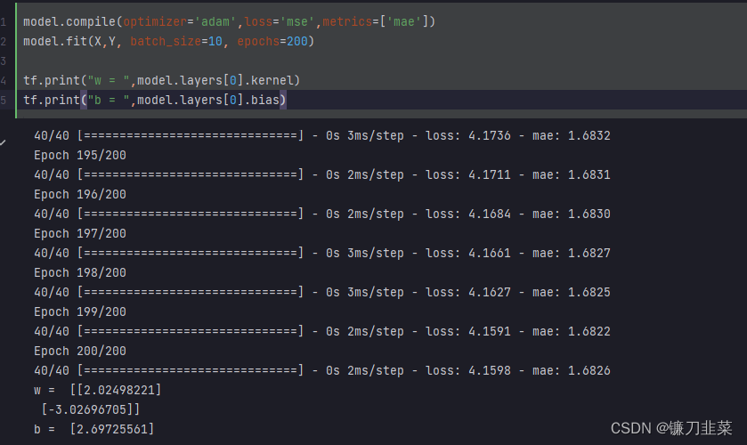
使用Sequential按层顺序构建模型，并使用内置model.fit方法训练模型（初级方法）：

定义模型

训练模型

使用fit方法进行训练：

DNN二分类模型

使用继承Model基类构建自定义模型，并构建自定义训练循环（高级方法）:

ds_train = tf.data.Dataset.from_tensor_slices((X[0:n*3//4,:],Y[0:n*3//4,:])).shuffle(buffer_size = 1000).batch(20).prefetch(tf.data.experimental.AUTOTUNE).cache()

ds_valid = tf.data.Dataset.from_tensor_slices((X[n*3//4:,:],Y[n*3//4:,:])).batch(20).prefetch(tf.data.experimental.AUTOTUNE).cache()

定义模型

tf.keras.backend.clear_session()


class DNNModel(models.Model):
    def __init__(self):
        super(DNNModel, self).__init__()

    def build(self, input_shape):
        self.dense1 = layers.Dense(4, activation="relu", name="dense1")
        self.dense2 = layers.Dense(8, activation="relu", name="dense2")
        self.dense3 = layers.Dense(1, activation="sigmoid", name="dense3")
        super(DNNModel, self).build(input_shape)

    # 正向传播
    @tf.function(input_signature=[tf.TensorSpec(shape=[None, 2], dtype=tf.float32)])
    def call(self, x):
        x = self.dense1(x)
        x = self.dense2(x)
        y = self.dense3(x)
        return y


model = DNNModel()
model.build(input_shape=(None, 2))

model.summary()

模型概览：

Model: "dnn_model"
_________________________________________________________________
 Layer (type)                Output Shape              Param #   
=================================================================
 dense1 (Dense)              multiple                  12        
                                                                 
 dense2 (Dense)              multiple                  40        
                                                                 
 dense3 (Dense)              multiple                  9         
                                                                 
=================================================================
Total params: 61
Trainable params: 61
Non-trainable params: 0
_________________________________________________________________

训练模型

自定义训练循环：

optimizer = optimizers.Adam(learning_rate=0.01)
loss_func = tf.keras.losses.BinaryCrossentropy()

train_loss = tf.keras.metrics.Mean(name='train_loss')
train_metric = tf.keras.metrics.BinaryAccuracy(name='train_accuracy')

valid_loss = tf.keras.metrics.Mean(name='valid_loss')
valid_metric = tf.keras.metrics.BinaryAccuracy(name='valid_accuracy')


@tf.function
def train_step(model, features, labels):
    with tf.GradientTape() as tape:
        predictions = model(features)
        loss = loss_func(labels, predictions)
    grads = tape.gradient(loss, model.trainable_variables)
    optimizer.apply_gradients(zip(grads, model.trainable_variables))

    train_loss.update_state(loss)
    train_metric.update_state(labels, predictions)


@tf.function
def valid_step(model, features, labels):
    predictions = model(features)
    batch_loss = loss_func(labels, predictions)
    valid_loss.update_state(batch_loss)
    valid_metric.update_state(labels, predictions)


def train_model(model, ds_train, ds_valid, epochs):
    for epoch in tf.range(1, epochs + 1):
        for features, labels in ds_train:
            train_step(model, features, labels)

        for features, labels in ds_valid:
            valid_step(model, features, labels)
        logs = 'Epoch={},Loss:{},Accuracy:{},Valid Loss:{},Valid Accuracy:{}'

        if epoch % 100 == 0:
            print('=======' * 10)
            tf.print(tf.strings.format(logs,
                                       (epoch, train_loss.result(), train_metric.result(), valid_loss.result(),
                                        valid_metric.result())))

        train_loss.reset_states()
        valid_loss.reset_states()
        train_metric.reset_states()
        valid_metric.reset_states()

train_model(model, ds_train, ds_valid, 1000)

参考资料

[1] 《30天吃掉那只Tensorflow》