本文参照官网例子实现流域的提取,官方GitHub地址如下pyflwdir:
该工具包目前仅支持D8和LDD两种算法,在效率上具有较好的应用性,我用省级的DEM(30米)数据作为测试,输出效率可以满足一般作业需要。
环境environment.yml如下:
name: pyflwdir

channels:
  - conda-forge

# note that these are the developer dependencies,
# if you only want the user dependencies, see
# install_requires in setup.py
dependencies:
  # required
  - python>=3.9
  - pyflwdir
  # optional for notebooks
  - cartopy>=0.20
  - descartes
  - geopandas>=0.8
  - jupyter
  - matplotlib
  - rasterio
用到的utils.py的代码如下:
import matplotlib
import matplotlib.pyplot as plt
from matplotlib import cm, colors
import cartopy.crs as ccrs
import descartes
import numpy as np
import os
import rasterio
from rasterio import features
import geopandas as gpd

np.random.seed(seed=101)
matplotlib.rcParams["savefig.bbox"] = "tight"
matplotlib.rcParams["savefig.dpi"] = 256
plt.style.use("seaborn-v0_8-whitegrid")

# read example elevation data and derive background hillslope
fn = os.path.join(os.path.dirname(__file__), r"D:\CLIPGY.tif")
with rasterio.open(fn, "r") as src:
    elevtn = src.read(1)
    extent = np.array(src.bounds)[[0, 2, 1, 3]]
    crs = src.crs
ls = matplotlib.colors.LightSource(azdeg=115, altdeg=45)
hs = ls.hillshade(np.ma.masked_equal(elevtn, -9999), vert_exag=1e3)


# convenience method for plotting
def quickplot(
    gdfs=[], raster=None, hillshade=True, extent=extent, hs=hs, title="", filename=""
):
    fig = plt.figure(figsize=(8, 15))
    ax = fig.add_subplot(projection=ccrs.PlateCarree())
    # plot hillshade background
    if hillshade:
        ax.imshow(
            hs,
            origin="upper",
            extent=extent,
            cmap="Greys",
            alpha=0.3,
            zorder=0,
        )
    # plot geopandas GeoDataFrame
    for gdf, kwargs in gdfs:
        gdf.plot(ax=ax, **kwargs)
    if raster is not None:
        data, nodata, kwargs = raster
        ax.imshow(
            np.ma.masked_equal(data, nodata),
            origin="upper",
            extent=extent,
            **kwargs,
        )
    ax.set_aspect("equal")
    ax.set_title(title, fontsize="large")
    ax.text(
        0.01, 0.01, "created with pyflwdir", transform=ax.transAxes, fontsize="large"
    )
    if filename:
        plt.savefig(f"{filename}.png")
    return ax


# convenience method for vectorizing a raster
def vectorize(data, nodata, transform, crs=crs, name="value"):
    feats_gen = features.shapes(
        data,
        mask=data != nodata,
        transform=transform,
        connectivity=8,
    )
    feats = [
        {"geometry": geom, "properties": {name: val}} for geom, val in list(feats_gen)
    ]

    # parse to geopandas for plotting / writing to file
    gdf = gpd.GeoDataFrame.from_features(feats, crs=crs)
    gdf[name] = gdf[name].astype(data.dtype)
    return gdf
执行代码如下:
import rasterio
import numpy as np
import pyflwdir

from utils import (
    quickplot,
    colors,
    cm,
    plt,
)  # data specific quick plot convenience method

# read elevation data of the rhine basin using rasterio
with rasterio.open(r"D:\Raster.tif", "r") as src:
    elevtn = src.read(1)
    nodata = src.nodata
    transform = src.transform
    crs = src.crs
    extent = np.array(src.bounds)[[0, 2, 1, 3]]
    latlon = src.crs.is_geographic
    prof = src.profile

ax = quickplot(title="Elevation")
im = ax.imshow(
    np.ma.masked_equal(elevtn, -9999),
    extent=extent,
    cmap="gist_earth_r",
    alpha=0.5,
    vmin=0,
    vmax=1000,
)
fig = plt.gcf()
cax = fig.add_axes([0.8, 0.37, 0.02, 0.12])
fig.colorbar(im, cax=cax, orientation="vertical", extend="max")
cax.set_ylabel("elevation [m+EGM96]")
# plt.savefig('elevation.png', dpi=225, bbox_axis='tight')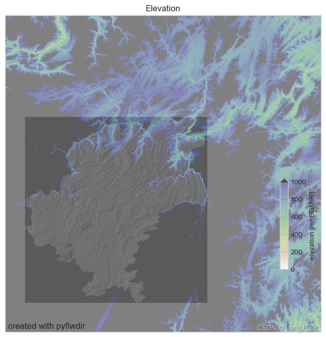
#####划分子流域
import geopandas as gpd
import numpy as np
import rasterio
import pyflwdir
# local convenience methods (see utils.py script in notebooks folder)
from utils import vectorize # convenience method to vectorize rasters
from utils import quickplot, colors, cm # data specific quick plot method
# returns FlwDirRaster object
flw = pyflwdir.from_dem(
data=elevtn,
nodata=src.nodata,
transform=transform,
latlon=latlon,
outlets="min",
)
import geopandas as gpd
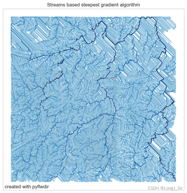
feats = flw.streams(min_sto=4)
gdf = gpd.GeoDataFrame.from_features(feats, crs=crs)
# create nice colormap of Blues with less white
cmap_streams = colors.ListedColormap(cm.Blues(np.linspace(0.4, 1, 7)))
gdf_plot_kwds = dict(column="strord", cmap=cmap_streams)
# plot streams with hillshade from elevation data (see utils.py)
ax = quickplot(
gdfs=[(gdf, gdf_plot_kwds)],
title="Streams based steepest gradient algorithm",
filename="flw_streams_steepest_gradient",
)
# update data type and nodata value properties which are different compared to the input elevation grid and write to geotif
prof.update(dtype=d8_data.dtype, nodata=247)
with rasterio.open(r"D:\flwdir.tif", "w", **prof) as src:
    src.write(d8_data, 1)

######################
#Delineation of (sub)basins#
###########
with rasterio.open(r"D:\flwdir.tif", "r") as src:
    flwdir = src.read(1)
    crs = src.crs
    flw = pyflwdir.from_array(
        flwdir,
        ftype="d8",
        transform=src.transform,
        latlon=crs.is_geographic,
        cache=True,
    )
    # define output locations
    #x, y = np.array([106.6348,26.8554]), np.array([107.0135,26.8849])
    #x, y = np.array([26.8554,106.6348]), np.array([26.8849,107.0135])
    x, y = np.array([106.4244,107.0443]), np.array([26.8554,27.0384])
    gdf_out = gpd.GeoSeries(gpd.points_from_xy(x, y, crs=4326))
    # delineate subbasins
    subbasins = flw.basins(xy=(x, y), streams=flw.stream_order() >= 5)
    # vectorize subbasins using the vectorize convenience method from utils.py
    gdf_bas = vectorize(subbasins.astype(np.int32), 0, flw.transform, name="basin")
    gdf_bas.head()

# plot
# key-word arguments passed to GeoDataFrame.plot()
gpd_plot_kwds = dict(
    column="basin",
    cmap=cm.Set3,
    legend=True,
    categorical=True,
    legend_kwds=dict(title="Basin ID [-]"),
    alpha=0.5,
    edgecolor="black",
    linewidth=0.8,
)
points = (gdf_out, dict(color="red", markersize=20))
bas = (gdf_bas, gpd_plot_kwds)
# plot using quickplot convenience method from utils.py
ax = quickplot([bas, points], title="Basins from point outlets", filename="flw_basins")
# calculate subbasins with a minimum stream order 7 and its outlets
subbas, idxs_out = flw.subbasins_streamorder(min_sto=7, mask=None)
# transfrom map and point locations to GeoDataFrames
gdf_subbas = vectorize(subbas.astype(np.int32), 0, flw.transform, name="basin")
gdf_out = gpd.GeoSeries(gpd.points_from_xy(*flw.xy(idxs_out), crs=4326))
# plot
gpd_plot_kwds = dict(
    column="basin", cmap=cm.Set3, edgecolor="black", alpha=0.6, linewidth=0.5
)
bas = (gdf_subbas, gpd_plot_kwds)
points = (gdf_out, dict(color="k", markersize=20))
title = "Subbasins based on a minimum stream order"
ax = quickplot([bas, points], title=title, filename="flw_subbasins")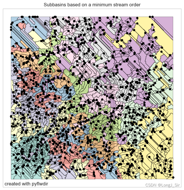
# get the first level nine pfafstetter basins
pfafbas1, idxs_out = flw.subbasins_pfafstetter(depth=1)
# vectorize raster to obtain polygons
gdf_pfaf1 = vectorize(pfafbas1.astype(np.int32), 0, flw.transform, name="pfaf")
gdf_out = gpd.GeoSeries(gpd.points_from_xy(*flw.xy(idxs_out), crs=4326))
gdf_pfaf1.head()

# plot
gpd_plot_kwds = dict(
    column="pfaf",
    cmap=cm.Set3_r,
    legend=True,
    categorical=True,
    legend_kwds=dict(title="Pfafstetter \nlevel 1 index [-]", ncol=3),
    alpha=0.6,
    edgecolor="black",
    linewidth=0.4,
)

points = (gdf_out, dict(color="k", markersize=20))
bas = (gdf_pfaf1, gpd_plot_kwds)
title = "Subbasins based on pfafstetter coding (level=1)"
ax = quickplot([bas, points], title=title, filename="flw_pfafbas1")
# lets create a second pfafstetter layer with a minimum subbasin area of 5000 km2
pfafbas2, idxs_out = flw.subbasins_pfafstetter(depth=2, upa_min=5000)
gdf_pfaf2 = vectorize(pfafbas2.astype(np.int32), 0, flw.transform, name="pfaf2")
gdf_out = gpd.GeoSeries(gpd.points_from_xy(*flw.xy(idxs_out), crs=4326))
gdf_pfaf2["pfaf"] = gdf_pfaf2["pfaf2"] // 10
gdf_pfaf2.head()
# plot
bas = (gdf_pfaf2, gpd_plot_kwds)
points = (gdf_out, dict(color="k", markersize=20))
title = "Subbasins based on pfafstetter coding (level=2)"
ax = quickplot([bas, points], title=title, filename="flw_pfafbas2")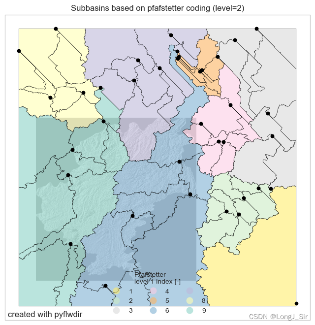
# calculate subbasins with a minimum stream order 7 and its outlets
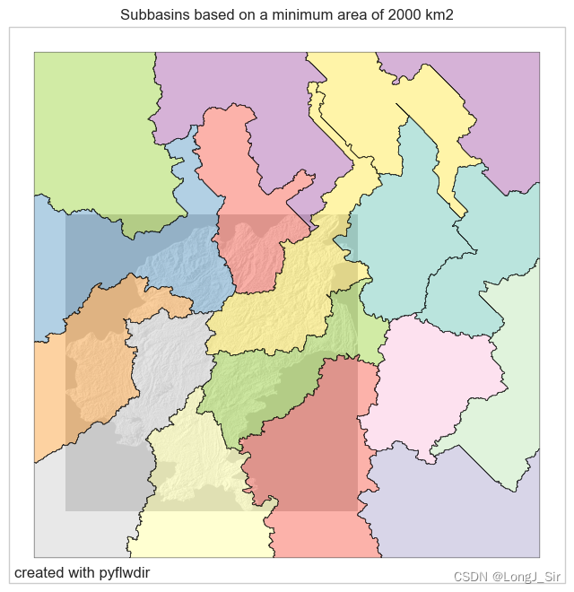
min_area = 2000
subbas, idxs_out = flw.subbasins_area(min_area)
# transfrom map and point locations to GeoDataFrames
gdf_subbas = vectorize(subbas.astype(np.int32), 0, flw.transform, name="basin")
# randomize index for visualization
basids = gdf_subbas["basin"].values
gdf_subbas["color"] = np.random.choice(basids, size=basids.size, replace=False)
# plot
gpd_plot_kwds = dict(
column="color", cmap=cm.Set3, edgecolor="black", alpha=0.6, linewidth=0.5
)
bas = (gdf_subbas, gpd_plot_kwds)
title = f"Subbasins based on a minimum area of {min_area} km2"
ax = quickplot([bas], title=title, filename="flw_subbasins_area")